Elat Sabhka Trenches
 Fig. 6e
Map of trenches T1 and T3 area detailing the locations of all other features in the figure (panels a-d).
click on image to open in a new tab
Kanari et al (2020)
- Fig. 1 Location Map from
Kanari et al (2020)
 Fig. 1
(a) Regional tectonic map of the Dead Sea Transform and location of the Gulf of Aqaba/Elat
(b) Topographic image map of the southern Arava Valley showing location of the study area of the Elat Sabkha. Previously mapped faults in black lines (after Garfunkel, 1970; Garfunkel et al., 1981; Sneh et al., 1998). Previous study sites including Avrona Sabkha and Yovata Sabkha and locations of the paleoseismic trenches (in block circles)
- QT = Qatar trench (Klinger et al., 2015)
- AT = Avrona Trenches (Amit et al., 1999; Zilberman et al., 2005)
- ST = Shehoret trenches (e.g. Amit et al., 2002)
- GAE = Gulf of Aqaba/Elat
CMP shots discussed in this study from seismic lines SI-4047 and GI-2108 are plotted as light-blue dots and yellow dots, respectively. The blue rectangle marks the extent of the study area maps presented in Figs. 3 and 9. The pink line represents the location of the offshore high-resolution seismic profile by Hartman et al. (2014) detailed in Fig. 2b.
Kanari et al (2020) - Fig. 2a Bathymetric Map from
Kanari et al (2020)
 Fig. 2a
Bathymetric map of the north end of the Gulf of Aqaba/Elat (Sade et al., 2008; Tibor et al., 2010) showing the location of faults on the shelf of the northern Gulf of Aqaba/Elat as mapped from interpretation of seismic reflection data (Hartman et al., 2014).
Kanari et al (2020) - Fig. 3a Fault Map from
Kanari et al (2020)
 Fig. 3a
The trace of the East Elat Fault and the Avrona Fault offshore (white lines) as mapped from seismic reflection data (after Hartman et al., 2014), and interpreted lineaments suspect as fault traces around the Elat Sabkha (yellow dashed lines) based on a pre-urbanization aerial photo from 1945 (Palestine Survey PS43–6003 and PS43–6017).
Kanari et al (2020) - Fig. 3b Fault Map from
Kanari et al (2020)
 Fig. 3b
The Avrona Fault offshore and the lineaments georeferenced to a modern satellite image, and the dataset used in the current study: location of seismic reflection profiles SI-4047 (light-blue circles mark CMP numbers), GI-2108 (yellow circles mark CMP numbers) and GI-2210 (blue line) and the paleoseismic trenches T1 and T3. The Hotel District of Elat is marked for reference to its vicinity to the surface rupture prone area. The seismic profiles are presented in Fig. 4.
Kanari et al (2020) - Fig. 9 Fault Map from
Kanari et al (2020)
 Fig. 9
The Avrona Fault, Avrona Fault Zone and active fault map based on the evidence for faulting presented in this study. The solid red line outlines the interpreted area with surface rupture evidence presented in this study from analysis of seismic reflection data (pink triangles) and the trench T3 fault zone (red star; location 34°58′29.86″E, 29°33′57.66”N). The area in dashed orange line is a suggested fault zone based on interpretation of our fault-potential lineaments presented in Fig. 3 (white dashed lines) and possible surface faulting deduced from the seismic reflection line GI2108 between CMPs 125–180 (pink triangles). See legend for details
Kanari et al (2020)
- Elat Sabkha Trench 1 area in Google Earth
 Elat Sabkha Trench 1 area
Trench location marked by a magenta line
click on image to explore this site on a new tab in Google Earth - Elat Sabkha Trench 3 area in Google Earth
 Elat Sabkha Trench 3 area
Trench location marked by a magenta line
click on image to explore this site on a new tab in Google Earth
Fig. 6e
Map of trenches T1 and T3 area detailing the locations of all other features in the figure (panels a-d).
click on image to open in a new tab
Kanari et al (2020)
 Fig. 6c
Liquefaction features and their spatial extent. (c) T1 liquefaction fluid escape structures (interpreted in yellow on photo) and its charcoal ET02 sample; white arrow points out liquefaction related feature.
Kanari et al (2020)
 Fig. 5b
Trench T3 log of the fault zone: The top 80 cm of the trench were disturbed by farming (marked by white dashed boundary). U1-U8 are stratigraphic units and F1-F11 are interpreted fault strands (see text for detail). Yellow hexagons mark charcoal samples locations; dated samples have adjacent radiocarbon age determinations presented. E1 and E2 are the interpreted event horizons which represent the faulting events (see text for detail). (b) The complete 0–7 m fault zone log; blue rectangle marks the area of panel (a); The presented log is simplified for clarity of the figure; a high-resolution more detailed log is available in the supplementary material SM1
Kanari et al (2020)
 Fig. 5a
Trench T3 log of the fault zone: The top 80 cm of the trench were disturbed by farming (marked by white dashed boundary). U1-U8 are stratigraphic units and F1-F11 are interpreted fault strands (see text for detail). Yellow hexagons mark charcoal samples locations; dated samples have adjacent radiocarbon age determinations presented. E1 and E2 are the interpreted event horizons which represent the faulting events (see text for detail). (a) detailed blow-up of the 3–5 m faulted strata in the fault zone
Kanari et al (2020)
 Fig. 6a
Liquefaction features and their spatial extent. (a) Trench log of Sand blow 1 structure (SB1) in T3 and its logged stratigraphic structure; boundaries of sand blow outlined in black dashed rectangle; L1-L7 are stratigraphic units of the West Sabkha (see text for detail). Yellow hexagons mark charcoal samples locations; dated samples have adjacent radiocarbon age determinations presented.
Kanari et al (2020)
 Fig. 6b
Liquefaction features and their spatial extent. (b) photo mosaic of Sand blow 2 structure (SB2) in T3; no detailed log is available for SB2
Kanari et al (2020)
Fig. 3bThe Avrona Fault offshore and the lineaments georeferenced to a modern satellite image, and the dataset used in the current study: location of seismic reflection profiles SI-4047 (light-blue circles mark CMP numbers), GI-2108 (yellow circles mark CMP numbers) and GI-2210 (blue line) and the paleoseismic trenches T1 and T3. The Hotel District of Elat is marked for reference to its vicinity to the surface rupture prone area. The seismic profiles are presented in Fig. 4.
Kanari et al (2020)
 Fig. 4a
Seismic line GI-2108 extending E-W on the southern part of the Elat Sabkha including interpretation of the Avrona Fault strands (yellow) and the Elat Fault (green); specific CMP points at interpreted fault strands are marked in red triangles (same CMPs are marked in Fig. 9).
Kanari et al (2020)
 Fig. 4c
High-resolution seismic line GI-2210 extending S-N on the eastern part of the Elat Sabkha including interpretation of the Avrona Fault strands (yellow); This line overlaps line SI-4047 (panel b) while the high resolution allows to identify fault offsets and deformation reaching up close to the surface. See Fig. 3 for location of the lines.
Kanari et al (2020)
 Fig. 4b
Seismic line SI-4047 extending S-N on the eastern part of the Elat Sabkha including interpretation of the Avrona Fault strands (yellow) and the Elat Fault (green); specific CMP points at interpreted fault strands are marked in red triangles (same CMPs are marked in Fig. 9).
- AF = Anticlinal Folds
- SF = Synclinal Folds
Kanari et al (2020)
 Fig. 2b
composite marine high-resolution seismic reflection profile across the gulf showing the six faults dividing the basin into the Elat sub-basin, Ayla horst, and Aqaba sub-basin (after Hartman et al., 2014). The location of the composite profile is marked in a pink line and the coastline of the GAE marked in black.
Kanari et al (2020))
 Fig. 8a
Radiocarbon age models for the deformation and liquefaction events in trench T3 using OxCal software: (a) OxCal modeled age for liquefaction event using samples from stratigraphic units L6 and L7 from SB1 and the liquefied sand from SB2
Kanari et al (2020)
 Fig. 8b
Radiocarbon age models for the deformation and liquefaction events in trench T3 using OxCal software: (b) OxCal modeled age for faulting events E1 and E2 using samples from stratigraphic units U0, U1, U4 and U5 from the fault zone. Model calculated using OxCal 4.3.2 and IntCal13 calibration curve (Bronk Ramsey, 2017; Reimer et al., 2013).
Kanari et al (2020)
 Fig. 7
Sediment accumulation rate estimation for trench T3: using the calibrated year BP ages of the radiocarbon ages from the bottom of the trench and the measured depth to the top of the trench, an accumulation rate was calculated. The triangles are radiocarbon ages with 2-sigma error bars and the solid lines are the linear interpolation regressions. The fault zone ages (blue) result in 0.9 mm/year accumulation rate, while the west sabkha SB1 ages (orange) result in 1.7 mm/year. Locations of charcoal samples on trench logs are presented in Figs. 5 and 6. Radiocarbon age determinations in Table 1.
Kanari et al (2020)
 Figure 2
Map of marine and continental data presented here: the submarine Avrona Fault mapped by Hartman (2015) in white line, paleoseismic trench locations (yellow lines), piston cores in red circles; Inset: blow-up of land survey data collections (trenches in yellow and GPR lines in black; GPR data not presented here); red star: the location of the fault observed in trench T3 (Fig. 3); red line: the suggested fault trace of the on-land Avrona Fault, traced between the edge of the submarine fault and the surface rupture of the 1068 AD and 1458 AD earthquakes observed in T3.
Kanari et al (2015)
 Figure 4
Grain size distribution (downcore spectrum of % volume per grain diameter) and 14C age determinations (cal BC/AD) of core P27 from the northern Gulf of Aqaba Elat. 14C age calibrated using Calib 7.0 (Stuiver and Reimer, 1993) and Marine13 calibration curve (Reimer et al, 2013).
Kanari et al (2015)
 Figure 5
Grain size distribution (downcore spectrum of % volume per grain diameter) of cores P17 (540 mbsl), P22 (316 mbsl) and P29 (282 mbsl) from the Northern Gulf of Aqaba-Elat; see Fig. 2 for core locations
Kanari et al (2015)
Fig. 6e(e) map of trenches T1 and T3 area detailing the locations of all other features in the figure (panels a-d). For the reader's convenience, a high-resolution version of the figure is available in the supplementary material SM2
Kanari et al (2020)
 Fig. 6d
Liquefaction features and their spatial extent. (d) liquefaction evidence from the 1995 Nuweiba M 7.2 earthquake, still visible today in the vicinity of T1; white arrow points out liquefaction related feature; photo taken in December 2011
Kanari et al (2020)
The cities of Elat, Israel and neighboring Aqaba, Jordan are major economic, cultural, and seaport centers. They are located on the northern shore of the Gulf of Aqaba/Elat (GAE) directly on the Dead Sea Transform. Yet the precise location of the fault trace and its tectonic activity are lacking. The interpretation of seismic reflection profiles across the GAE beach and paleoseismic trench data located 2.2 km north of the shoreline provide evidence that the active offshore mapped Avrona Fault extends onland along the eastern side of the Elat Sabkha (mudflat), where three prominent fault strands crosscut the sedimentary fill. Mismatch of reflector geometry across the faults and flower structures indicate strike-slip faulting with a normal-slip component. Subsurface data from two trenching sites provide evidence for a minimum of two surface ruptures and two paleoliquefaction events. Faulting is constrained by radiocarbon dating for an Event 1 between 897 and 992 CE and Event 2 after 1294 CE. We suggest that the historically documented 1068 CE, and at least one later earthquake in 1458 or 1588 CE, ruptured the Elat Sabkha site. Based on fault mapping, we suggest a minimum value of M 6.6 for the 1068 CE earthquake. Whereas no surface rupture was observed for the 1212 CE historical earthquake, fluidized strata radiocarbon dated to before 1269–1389 CE identified as paleoliquefaction may be attributed to it. Two liquefaction sand-blows mapped in the trench likely formed after 1337 CE and before 1550 CE, which possibly occurred at the same time as in the second faulting event. Our data suggest that no large event occurred along the Avrona segment in the past ~430–550 years. Given a ~ 5 mm/yr slip rate, we conclude that a significant period of time passed since the last surface rupturing on the Avrona Fault, increasing its seismic potential.
A key element of seismic hazard assessment is the characterization of seismogenic sources. The characterization of a seismic source involves detailed geologic and geophysical studies to exactly locate active faults and to determine the potential magnitude, rupture length, and recurrence of earthquakes on the fault. We investigate a strand of the Dead Sea Transform fault, known as the Avrona Fault, that has been mapped offshore in the Gulf of Aqaba/Elat (GAE) using seismic reflection data (Hartman et al., 2014, 2015) and to the north of the city using paleoseismic trenching (Amit et al., 1999, 2002). However, within the municipality of Elat, no active fault deformation or other evidence of past earthquakes has been previously documented.
The cities of Elat (Israel) and Aqaba (Jordan) are located at the north tip of the Gulf of Aqaba/Elat (the northeast extension of the Red Sea; Fig. 1). These cities are major economic, cultural, and recreational centers for southern Israel and Jordan, and vital aerial and marine ports. Both Elat and Aqaba are built on active plate boundary faults, which have ruptured in the past. Aqaba was completely destroyed in the 1068 CE earthquake (Ambraseys et al., 1994; Avner, 1993; Whitcomb, 1994; Guidoboni and Comastri, 2005; Ambraseys, 2009) and significant damage to structures in both Elat and Aqaba was inflicted by the Mw 7.2 1995 Nuweiba earthquake even though the epicenter was located ~90 km to the south (Hofstetter, 2003). During that event, liquefaction occurred in the cities of Elat and Aqaba, both in artificial fillings and in natural sabkha and coastal deposits (Wust, 1997), and subsequent geotechnical studies showed that the coastal zone is susceptible to liquefying (Mansoor et al., 2004; Abueladas, 2014; Abueladas et al., 2020). Clearly, assessment of seismic hazard in these neighboring cities is vital. Aqaba and Elat are located on a transition zone between two structural realms at the southern part of the Dead Sea Fault system (DSF): the deep en echelon submarine basins of the Red Sea (Ben-Avraham, 1985) and the shallow continental basins of the Arava (ten Brink et al., 1999), localizing into a single fault strand farther northward. A report (Wieler et al., 2017) followed by a recent webpage created by the Geological Survey of Israel ( Geological Survey of Israel – High-resolution mapping of Elat) details earthquake hazards and mapped active faults in the Elat region (including results from this current study).
We aim to identify and locate the active faults in the Elat/Aqaba region, and especially within the boundaries of Elat itself, and estimate their seismogenic potential for earthquake hazard assessment. Given these goals, we analyze previously unpublished seismic reflection profiles that were collected across and along the Elat Sabkha and provide evidence for the neotectonic history of faulting. We also report on the first paleoseismic investigations in the city of Elat, within the Elat Sabkha and provide evidence of paleoearthquake ground rupture and liquefaction. By correlating the recently mapped offshore Avrona Fault (Hartman et al., 2014) with the onshore fault in Elat from both paleoseismic trenching and seismic reflection profiling, the seismic hazard potential of these faults can be better characterized within the heavily urbanized Elat city and its very closely neighboring Aqaba city.
The Gulf of Aqaba/Elat (GAE) and the 160-km long Arava Valley (Wadi ‘Arabah) northeast of the cities of Elat and Aqaba formed along the Dead Sea Transform (DST) plate boundary that separates the Sinai subplate from the Arabian plate (Fig. 1a). Quaternary slip rate estimates of the DST vary between 2 mm/yr and 10 mm/yr based on offset drainage systems along the Avrona and Arava fault segments (Zak and Freund, 1966; Garfunkel et al., 1981; Ginat et al., 1998; Klinger et al., 2000; Niemi et al., 2001). For details of different sources of data for these studies see Table 1 in Le Beon et al. (2008). Geophysical data indicate that the GAE developed from an en echelon array of three basins formed between left-stepping, strike-slip faults (Ben-Avraham et al., 1979; Ben-Avraham, 1985). Gravity data (ten Brink et al., 1999) indicate that the northernmost basin of the GAE, called the Elat Deep, extends on land beneath the Elat Sabkha and Avrona Playa. En echelon basins extend northward from the GAE into the Timna/Yovata/Taba Playa, the Dead Sea, and the Sea of Galilee (e.g. Garfunkel, 1981).
Previous studies of the submarine structure of the northern GAE suggest that slip on the eastern and western boundary faults is predominantly normal and that both faults are active (Ben-Avraham et al., 1979; Ben-Avraham, 1985; Ben-Avraham and Tibor, 1993). However, recent high-resolution seismic reflection and bathymetric data (Tibor et al., 2010; Hartman, 2012; Hartman et al., 2014, 2015) revealed a complex fault system across the shelf of the northern GAE with varying degrees of recent fault activity. The GAE shelf (Fig. 2) can be divided into three structural fault blocks (Tibor et al., 2010).
Based on high-resolution seismic reflection data, Makovsky et al. (2008) and Hartman et al. (2014) suggest that the recently active segment in the northern GAE is the Avrona Fault with a left-lateral, slip rate of 0.7 ± 0.3 mm/yr in the Late Pleistocene and 2.3–3.5 mm/yr during the Holocene. Two intrabasinal faults east of the Avrona Fault have been inactive for the last several tens of thousands of years (Fig. 2) and motion from these faults has likely transferred to the Avrona Fault (Hartman et al., 2014). Hartman et al. (2014) calculate a Holocene vertical slip rate of 1.0 ± 0.2 mm/yr for the Elat Fault and 0.4 ± 0.1 mm/yr for the Aqaba Fault. These authors suggest that the geometry, slip rates, and slip history of the faults on the shelf show the following: 1) during the Late Pleistocene, several intrabasinal faults became dominant across the basin, and 2) during the Holocene, the submarine Avrona Fault accommodates most of the strike-slip faulting in this transform plate boundary setting.
The Arava Valley (Wadi ‘Arabah), striking northeast from the GAE shoreline, is a structural and topographic valley delimited along much of its margins by normal faults (e.g. Garfunkel et al., 1981; Ibrahim, 1991; Rashdan, 1988). The valley is crossed by the active, NNE-striking Avrona Fault segment in the south and the Arava fault segments in the north along the DST (Garfunkel et al., 1981). The long-term slip rate of about 4.5 ± 1.5 mm/yr on the Arava fault is in agreement with geodetic estimates of the current horizontal plate motion along the DST suggested to be 3.7–7.5 mm/yr (Wdowinski et al., 2004; Ostrovsky, 2005; Le Beon et al., 2008).
The Elat fault system consists predominantly of normal faults that juxtapose Pleistocene alluvial fan sediments and Holocene deposits. Garfunkel (1970) traced a fault that he named the Elat Fault along the western Elat Sabkha and the western coast of the northern GAE and mapped a branch of that fault along a bathymetric escarpment in the GAE. Shaked et al. (2004, 2012) interpreted the submergence and burial of coral reefs and archaeological campsites along the western coastline of Elat as evidence of earthquakes and related tsunami sediment transport. One event ~2300 yr BP was corroborated by tsunami deposits along the northern portion of the GAE (Goodman Tchernov et al., 2016). Shaked et al. (2004, 2012) suggested that slip along a segment of the western boundary normal fault caused subsidence of 1.8 m in two earthquakes in the past 5000 yr BP.
Paleoseismic studies of the Avrona Fault some 15–25 km farther north revealed slip on normal faults across the valley fill (Gerson et al., 1993; Amit et al., 1995, 1996, 1999; Enzel et al., 1996; Porat et al., 1996, 1997; Shtivelman et al., 1998) and on the Avrona strike-slip fault (Amit et al., 2002; Zilberman et al., 2005). Additionally, a historical rupture on the Avrona Fault at the Avrona Sabkha site is attributed to the 1068 CE earthquake. Paleoseismic studies on the Avrona Fault at the south end of the Yotvata (Taba) Sabkha, about 30 km north of Aqaba, are reported by Allison (2013) and Klinger et al. (2015). Klinger et al. (2015) report two fault zones were observed in the trench about 10 m apart. They identified a conservative minimum of six paleoearthquakes. Radiocarbon dating indicated that the time window exposed in the trench extends from present to 4000 yr BP, with clustered seismic activity between the 7th and the 15th century, around 2000 yr BP and between 3000 yr BP and 4000 yr BP.
Aerial photos from the 1945 PS (Palestine Survey PS43-6003 and PS43-6017) at a scale of 1:50,000 were used to map lineaments that are potentially locations of active fault surface rupture (Fig. 3). Lineaments on the 1945 air photo were based on colour, textural, and tonal differences. These interpretations were saved as a lineament file and projected onto the high resolution orthophoto of the city provided by the Elat municipality.
Based on the interpretation of aerial photos (Fig. 3) and the onshore projection of the submarine Avrona Fault as mapped from marine seismic reflection data (Hartman et al., 2014), a 90-m-long paleoseismic trench, T1, was excavated on the palm orchards of Kibbutz Eilot, about 1 km north of the Elat shoreline (Fig. 3b). Trench T1 revealed liquefaction features, but the fault trace itself was not found. We then excavated a 70-m-long trench, T2, approximately 600 m farther north of T1, but this trench was quickly abandoned without further study due to a very shallow ground water table only 20–30 cm below the ground surface. A third trench, T3, was excavated 1200 m farther north from T1 (2.2 km from the shoreline) in an agricultural field. Trench T3 was 300 m long, and at the western part of it, the active trace of the Avrona Fault was found and documented (Fig. 5). The depth of the trench was limited to 1.1 m to 1.2 m because of the shallow water table. The trenches were excavated using a backhoe and their walls were cleaned, photographed, and logged using standard paleoseismologic methods (e.g. McCalpin, 2009).
Interpretation of the 1945 aerial photographs indicates that the Elat Sabkha is a coastal mudflat that extends from the shoreline to approximately 2.8 km inland where it appears to border the Roded alluvial fan and probably interfingers with it in the subsurface (Fig. 3). The sabkha developed along the outlet of the SSW-draining Arava valley where it empties into the Gulf of Aqaba/Elat. In the 1945 aerial photo, multiple anastomosing to gently meandering channels can be seen crossing the sabkha (Fig. 3a). Today, these channels collect into one canal to the east of the main hotel district (around CMP 75 of line GI2108 in Fig. 3b). The margins of the sabkha are marked by distinct, NE-trending lineaments (marked in yellow in Fig. 3a). The westernmost lineament appears to be the boundary between older and younger alluvial fans previously identified as the location of the Elat Fault (e.g. Garfunkel et al., 1981; Gerson et al., 1993). On the eastern side of the sabkha are three subparallel lineaments marking the boundary between different zones of the sabkha based on their appearance (colour and texture) in the aerial photo. We interpret the eastern border of the Elat Sabkha as the location of the Avrona Fault zone as was also suggested by previous authors (e.g. Garfunkel, 1970; Garfunkel et al., 1981; Amit et al., 2002). We excavated our trenches T1 and T3 there (pink lines in Fig. 3b).
The sediment exposed in Trench T3 shows a sequence of shallow, sand-filled channels and overbank floodplain and mudflat deposition (Fig. 5). Laterally migrating and gently aggrading channel fill is typical for the eastern portion of the trench. The channels are approximately 2 m wide and 30 cm deep. They are filled with predominantly fine- to medium-grained sand with cross-bedding that indicates east-west oscillations of the channel's margins. Point bar cross-beds are often draped by mud at their tops suggesting an original depositional dip for some fine-grained units in the trench. The western portion of the trench is dominated by interbedded sand, silt, and clay layers interpreted as flooding events. Beds of laminated mud and silt suggest periods of standing water. The uppermost 80 cm were anthropogenically disturbed due to deep agricultural plowing (Fig. 5).
The fault zone in Trench T3 is 9 m wide and consists of eleven fault strands that terminate upward at different stratigraphic levels that suggest two possible surface rupturing events. Fault F11 is the easternmost fault. Faults F1-F4 are a series of upward-branching strands of one fault trace with very little observed vertical displacement of up to 1.5 cm and a slight push-up geometry. Fault F11 is insufficiently mapped due to the lack of fine-grained interbeds to provide much detailed history of faulting at this location. F5 and the combined F6/F7 have normal components across them with down-to-the-west offset of apparent 10 cm and up to 15 cm, respectively. F8 has 12 cm of down-to-the-west, apparent vertical separation. Total apparent vertical separation across F3 to west of F8 is 43 cm measured for the change of elevation of clayey silt layer U2. F9 shows apparent vertical offset of 7 cm down-to-the-west at the top of a silty-sand layer, but the trench floor interferes with tracing it further down. F10 is above the anthropogenic disturbance zone and thus has significant uncertainty in its mapping and interpretation. There is apparent vertical change on both sides of F11, but with insufficient evidence to identify the faulting history. If the original topography of the ground prior to faulting had a ridge and swale morphology as is common in a fluvial environment, then lateral slip on faults would cause apparent vertical separation of stratigraphic units. Furthermore, if there are rapid lateral changes in stratigraphic thickness of units in the depositional environment, then strike-slip on a fault would also cause apparent vertical offsets. Because the apparent offsets are all down-to-the west (except F11), this could indicate that there is a component of normal slip on the faults.
Below the anthropogenic disturbance (plow zone), we define eight marker layers (units U1-U8) across the faulted portion of the trench (Fig. 5). Layer thickness of units varies across the fault traces. This is especially true for Units U3 and U4. U5 has distinct notable variation in thickness across this strand. Furthermore, mismatch of layer thickness across the fault strands suggests strike-slip fault motion as would be expected for the Avrona Fault. The layered stratigraphy in the upper interfurrow segment suggests that F5 fault rupture terminates in unit U1. Given what we can discern from the overlying stratigraphy within the interfurrows, we posit that faults F1-F7 offset units U2-U8 in an event labeled E1. Faults F11 and F1–7 appear to terminate in the sand of U1 below or near the anthropogenic disturbance zone. These data indicate a possible surface rupture event after the deposition of U2 and before deposition of the silt layer in the U1 sand layer (Fig. 5). As the silt layer in U1 (radiocarbon sample ET3–122 dated at with a 2-sigma calibrated age of 1023–1248 CE) does not directly cap the faults, but is the uppermost last continuous unit below the anthropogenic disturbance zone, we have utilized this as the post-event horizon. However, radiocarbon analyses of samples 130 and 131 that are stratigraphically above this layer, within the zone between furrows, were used in the age model as described below.
Stratigraphically above the Units U1-U8 and to the west are younger layers of the sabkha (Fig. 5). Units U1B (silt) and U1A (clay) were deposited above the U1 sediment. These units and older U1-U8 units appear to dip gently to the west. Given the appearance of the dipping clay strata on the migrating channel deposits exposed to the east and the sedimentary contact to migrating point bar sequence in a channel, we interpret the dip of these layers to be tectonic. Within a predominantly flat-lying, aggrading depositional environment, the approximate 5–10 degree dips indicate tectonic tilting or folding. The dipping units appear west of F5, F6/7, and F8. U1B and U1A have an apparent vertical offset of 12 cm across F8. It is not clear whether the silt and clay layers above F5-F7 in the interfurrow area is equivalent to U1B and U1A. If they are, then F6–7 likely extends higher in the stratigraphic section and would post-date motion on F5 (E1). The upper termination of F8 is not known because of the deep plowing. However, based on the given data, it appears that F8 cuts higher in the stratigraphic section than F1-F5. Faults F9-F10 offset Units 1B and 1A and sand, silt, and clay layers that are stratigraphically younger. We do not have any stratigraphic control of the capping layer of this proposed event (E2).
Given the limitation of the dataset due to anthropogenic modification of the site, we interpret at least two fault ruptures in Trench T3. We interpret the trench data as:
- the first event (E1) ruptures units U2–U8 (F1–F5, and possibly F11)
- deposition of units U1B and U1A and overlying layers in the accommodation space created by down-to-the west faulting
- second event (E2) on F6/F7 and/or F8–F10
The size, frequency, and distance from an epicenter of earthquake-induced liquefaction features depend largely on the strength of the ground motion, a high water table, and the presence of soil susceptible to liquefy (e.g. Tuttle et al., 2019). The 1995 rupture of a submarine fault of the DST system in the Gulf of Elat/Aqaba in the Mw 7.2–7.3 Nuweiba earthquake (Dziewonski et al., 1997; Hofstetter, 2003) about 90 km southwest of Elat created liquefaction sand blows in the city (Wust, 1997). These sandblows are still visible on the ground surface (Fig. 6). In this study, we document evidence for paleoliquefaction in our trench exposures.
Two liquefaction structures (Fig. 6a, b), rather large in size (up to 5 m in diameter and 1 m high) were documented in Trench T3 west of the location of the fault rupture. A representative section of the stratigraphy composed of 7 main units (L1-L7) is presented in the log (Fig. 6a). A large liquefaction sand blow (SB1) is mapped as a mound of unstratified sand which seems to have torn through and carried some of the silt, clay and clayey silt layers as rip-up clasts within the sand and has deposited these layers away from the center of the feature. The boundaries of SB1 are outlined in black dashed rectangle in Fig. 6a. Layer (L3) caps the SB1 liquefaction feature. Sand blow 2 (SB2) has a similar construction with a mound of unstratified sand flanked by fine-grained sediment sloping away from the vent (Fig. 6b). The feeder dikes for each of these features was not identified. We interpret this as evidence for liquefaction at shallow depth and not a deep-sourced injection type. Radiocarbon samples within the sand blow provide a minimum age of formation of ~400 years BP as detailed below.
Trench T1 (Fig. 6) revealed liquefaction deformation features but no fault trace was evident. The uppermost unit A is disrupted by modern agriculture similar to the plow furrows observed in Trench T3. Below Unit A is a sand unit (Unit B; no sharp boundary or difference between them but the disrupted soil in unit A) and a laminated unit of alternating silt and clay (Unit C). Unit D contains interbedded layers of medium-grained sand with ripple laminations, coarse sand lenses, and very fine sand. Clear evidence of fluid escape structures is evident (Fig. 6c). This includes contorted and disrupted beds and ball-and-pillar structures in Unit D. This layer is capped by the flat-lying Unit C layer. Radiocarbon dating of unit C provides a maximum age for the interpreted liquefaction feature.
A total of 12 charcoal samples were collected from Trench 1 and Trench 3 and were sent for radiocarbon analyses (Table 1). Radiocarbon ages were corrected for isotope fractionation and calibrated using the Calib 7.1 software (Stuiver et al., 2019). A sediment accumulation rate was calculated for deposits in Trench 3 at the fault zone and in the west sabkha near the sand blow locations (Fig. 7). Using the depth and ages of three lower radiocarbon results at the fault zone, a sedimentation rate of 0.9 mm/yr was calculated. At the location of the sand blow, using the depth and ages of the lower two radiocarbon samples yielded a 1.7 mm/yr sediment accumulation rate. These data suggest that subsidence and accommodation space within the Avrona Sabkha and fault zone varies by a factor of about two.
Age modeling using the OxCal program and the IntCal13 calibration curve (Bronk Ramsey, 2017; Reimer et al., 2013) was performed for the radiocarbon results and combined with stratigraphic data from the faulted section of T3. Units U8-U2 were deposited before an earthquake that appears to be capped by layers in the lower unit U1. Radiocarbon samples ET3–120 (U5), ET3–121 (U4), ET3–132 (U2) are below the event and ET3–122, ET3–131, ET3–130, and ET3–133 are above it (Fig. 5). Reiterative OxCal model runs for the above sequence identified three samples in poor agreement that were removed. The final OxCal age model included samples ET3–120, ET3–130, ET3–131, and ET3–133 as presented in Fig. 8. The 2-sigma age model result indicates that the first faulting event (E1) occurred between 897 and 992 CE, and the second faulting event (E2) occurred after 1287 CE. The agricultural plowing of the top of the trench prevents the dating of the cap. The historical records rule out significant earthquake surface ruptures in this location in the past ~450 years (e.g. Klinger et al., 2015).
Two liquefaction features at the same stratigraphic level were documented in the western portion of Trench T3 (Fig. 6). These features are interpreted to be earthquake-induced liquefied sand. The features are capped by flat-lying strata that lack radiocarbon age dating. One radiocarbon sample (ET3–135) yielded an age of 2133–1903 BCE. We suspect it is a remobilization of charcoal older than all other C-14 results for this trench. The process of liquefaction can fluidize saturated sands at depth and inject these to the surface. Three radiocarbon samples (ET3–124, ET3–123, and ET3–134) were collected from under and within the sand blows and thus pre-date the causative earthquake. Utilizing these ages below a boundary event in the OxCal modeling program indicated that ET3–134 was in poor agreement, and it was removed from the model. With the remaining two radiocarbon dates, a probability distribution for the age of liquefaction of 1294–1635 CE was obtained. If we use the sediment accumulation rate of 1.7 mm/yr and the depth to the capping horizon of 70 cm, then the capping layer (L3) began forming approximately 400 years ago. This would suggest that the sand blow formed before 1550 CE.
In Trench T1 (Fig. 6), a dewatering structure that is likely due to seismically-induced liquefaction is capped by laminated sediment of Layer C. The charcoal sample from this layer (ET02) yielded split sample radiocarbon ages of 690 ± 25 and 675 ± 25 (Table 1). The calendar age range for these two samples is 1269–1389 CE indicating that the liquefaction event occurred sometime before the late 13th to late 14th centuries.
Haynes et al. (2006) infer from historical earthquake intensity data that major post-sixth century earthquakes probably occurred in the Wadi Araba and Dead Sea Fault in 634, 659/660, 873, 1068, 1212, 1293, 1458, 1546, and 1588 CE (Russell, 1985; Ben-Menahem, 1991; Ambraseys et al., 1994; Amiran et al., 1994; Guidoboni et al., 1994; Guidoboni and Comastri, 2005; Ambraseys, 2009). Klinger et al. (2015) narrow the largest well documented events of the southern DST after the eighth century to 1068, 1212, 1293, and 1458 CE. The surface rupture events, E1 and E2, that we document in the Elat Sabkha trench T3 appear to best correlate with the 1068 CE and 1458 CE historical earthquakes.
Klinger et al. (2015) radiocarbon dated ruptures at the Qatar site (Yotvata/Taba/Timna Sabkha), 30 km north of Elat and Aqaba, in the historical earthquakes of 1068 CE, 1212 CE, and 1458 CE, and two other earlier earthquakes in 746–757 CE and 363 CE. They suggest that the surface rupture of the 1068 CE earthquake terminated somewhere close to the Yotvata Sabkha and their Qatar trench site (Fig. 1b). Our data of surface rupture in the Elat Sabkha brings new evidence for southward continuation of the 1068 CE faulting, which was identified by Zilberman et al. (2005) in the Avrona Sabkha further north. We confirm the hypothesis by Klinger et al. (2015) about the southward continuation of the fault.
The rupture length of the 1068 CE earthquake fault can be constrained by the current study, documentation of rupture at the Avrona Sabkha (Zilberman et al., 2005), and the observations by Klinger et al. (2015). If we combine the 35 km of rupture onland from Qatar trench in the Yotvata Sabkha to trench T3 in Elat with the mapped offshore length of the fault 2 km further south from the coast (Hartman et al., 2014), a minimum of 37 km likely ruptured in the 1068 CE earthquake. Using the empirical relationship between fault rupture length and magnitude of Wells and Coppersmith (1994), we suggest a magnitude of M 6.6–7.1 for the 1068 CE earthquake. Historical accounts report massive destruction in the ancient Islamic city of Ayla in 1068 (Guidoboni and Comastri, 2005; Ambraseys, 2009). Compelling evidence for earthquake damage is confirmed by archaeological excavation of the Ayla site in Aqaba (Whitcomb, 1994). A reported possible tsunami in 1068 CE also supports a partial offshore rupture and/or seismically- induced submarine slump failures. Our results refute the location suggested by Ambraseys and Melville (1989) who located the 1068 CE event in NW Saudi-Arabia.
No earthquake rupture evidence was observed for the 1212 CE earthquake in the current study. Klinger et al. (2015) suggested that the rupture segment of the 1212 CE earthquake extends from the Qatar trench site south to the northern Gulf of Aqaba/Elat, thus to the T3 and T1 trench site. Klinger et al. (2015) report that this earthquake produced extensive damages to the city of Ayla and was widely felt in Egypt and reported north in the Wadi Araba (Ambraseys, 2009). A brecciated layer is associated to this event in the Dead Sea basin (Kagan et al., 2011), but no ground rupture related to this event was identified at the trench site of Qasr Tilah, located near the south boundary of the Dead Sea basin (Haynes et al., 2006). This leads us to suggest that either the 1212 CE faulting might have occurred elsewhere on another fault strand in the Elat Sabkha and not in the fault zone documented in trench T3, or possibly, the surface faulting did not extend as far south as Elat. Zilberman et al. (2005) suggest that the stronger earthquake of 1068 CE seems more likely to have caused the severe damage and surface rupture of the Avrona Sabkha area than the weaker 1212 CE earthquake. This supports an above assumption that the 1212 CE earthquake did not rupture the Avrona Fault. However, Guidoboni and Comastri (2005, p. 233-234) write that the primary source for this earthquake is Abu Shama from Damascus who wrote: "The most violent shock was at Aylat, on the coast." This is the city of Aqaba. It is possible that the location of the earthquake rupture for the 1212 CE earthquake is a submarine segment of the fault in the northern Gulf of Aqaba/Elat. This could suggest that fine, cm-scale fracturing may be created by seismically induced ground motion rather than surface rupture at the Qatar site.
Paleoliquefaction in the T1 trench may be related to the 1212 CE earthquake. Fluidized sediments that are likely mobilized by seismic shaking are capped by a flat-lying thinly bedded to laminated deposit of clayey silt and very fine sand (Fig. 6c). This layer is radiocarbon dated to 1269–1389 CE and was deposited after an earthquake. Therefore, the T1 paleoliquefaction may be evidence for the 1212 CE earthquake or even the 1068 CE earthquake in the Elat Sabkha.
Klinger et al. (2015) suggests that the 1458 CE earthquake ruptured a section of the Wadi Araba fault located between their site and the southern tip of the Dead Sea, while the current study suggests that an event post-dating 1287 ruptured the surface at the T3 trench in Elat. Klinger et al. (2015) suggest that there is no mention of significant damage to Aqaba in this period, and therefore inferred that the earthquake ruptured to the north in the central Wadi Araba. Zilberman et al. (2005) also do not report surface ruptures of this event in the Avrona Sabkha. It is possible that our E2 surface rupture is the earthquake of 1588 CE that was felt in northwest Arabia, Ayla, and Cairo (Ambraseys, 2009). Ambraseys and Melville (1989) placed the epicenter of this event in northwest Arabia. Klinger et al. (2015) do not find evidence for the 1588 CE earthquake surface rupture in their study area. Given the poor age constraints on the upper limit of the timing of faulting, we are unable to differentiate between the historical earthquakes of 1458 CE and 1588 CE. Our paleoliquefaction sand blows (SB1 and SB2) suggest that this earthquake occurred after 1287 CE and possibly before 1550 CE if we use a sediment accumulation rate to calculate the age of burial of the feature. These data tend to support an interpretation of 1458 CE, but are inconclusive.
In summary, the paleoseismic data suggest:
- a faulting event (E1) in 897–992 CE
- a liquefaction event sometime before 1269–1389 CE, which could be the same as E1 or a different event
- a faulting event (E2) after 1294 CE
- a liquefaction event after 1337 CE and possibly before 1550 CE, which may have occurred at the same time as faulting event E2, or in a different earthquake
Our data suggest that either the 1458 CE or 1588 CE ruptured the Avrona Fault in the Elat Sabkha. Our data suggest that no large event occurred along the Avrona segment in the past ~550 years following the 1458 CE earthquake or 430 years following the 1588 CE earthquake. Given either scenario, it has been a significant period of time since the Avrona Fault has experienced a surface rupturing earthquake. Using a slip rate of 4.7 mm/yr (Niemi et al., 2001) for the DST, an estimated 1.9–2.6 m of strain has already accrued.
Evidence for active faulting and recent earthquake history within the city of Elat along the southern Dead Sea Transform (DST) fault system shows the importance of combining all available data from onshore and offshore for investigating seismic hazard at coastal environments. Along the eastern margin of the Elat Sabkha, seismic reflection data reveal that the main Avrona Fault is a continuous, through-going strike-slip fault that connects the location of the offshore fault on the GAE continental shelf, to the trench T3 site, and 3 km inland to the CMP 419 on the north-south oriented SI-4047 seismic line. This fault is active and the flower-structure geometry indicates that it is predominantly a strike-slip fault. Two additional faults in the Elat Sabkha west and east of the main strand and likely subparallel to it define a 750-m-wide fault zone. The West Avrona Fault is vertical and parallel or subparallel to the main strand. The East Avrona Fault may have left-oblique normal slip. The data indicate syntectonic deposition and growth strata thickening toward the southwest and into the offshore marine basin.
The first paleoseismic trenching within the boundaries of Elat city identified the location of the on-land Avrona active fault within the Elat Sabkha. Connecting it to the offshore mapped fault places the Avrona Fault along a N20°E trend and extending approximately 2.2 km inland from the shoreline. We conclude that this is a capable active fault, which underlies the Hotel District of Elat city.
Evidence for surface rupture in two earthquakes is observed in the Elat T3 Trench. Radiocarbon dating suggests the two faulting events may correlate to the 1068 CE and 1458 or 1588 CE (the first better supported by sediment accumulation rate). The time constraints prevent an unequivocal distinction between the earthquakes of 1458 CE and 1588 CE. Hence, a third earthquake rupture cannot be excluded.
No earthquake surface rupture was observed for the 1212 CE earthquake in the current study. However, fluidized strata radiocarbon dated to before 1269–1389 CE may be evidence for the 1212 CE earthquake. The Elat Sabkha has a potential for recovering records of past liquefaction events. Two sand blows mapped in trench T3 may have occurred at the same time as in the second faulting event (either 1458 CE or 1588 CE).
Our data suggest that a minimum of 37 km likely ruptured in the 1068 CE earthquake, which corresponds to an M 6.6–7.1 earthquake, and ~430–550 years of quiescence, entailing a significant accumulation of strain. Together these data indicate a high seismic hazard in the greater Elat-Aqaba region.
Supplementary data to this article can be found online at https://doi.org/10.1016/j.tecto.2020.228596.
Kanari et al. (2020:13), assuming Event E1 corresponds to the 1068 CE earthquake, estimate a minimum rupture length of ~37 km and derive a magnitude of M = 6.6–7.1 using a scaling relationship from Wells and Coppersmith (1994). This suggests a local intensity of VIII (8).
Minimum intensity for a surface rupturing earthquake is VII (7).
- Earthquake Archeological
Effects from Rodríguez-Pascua et al (2013: 221-224)
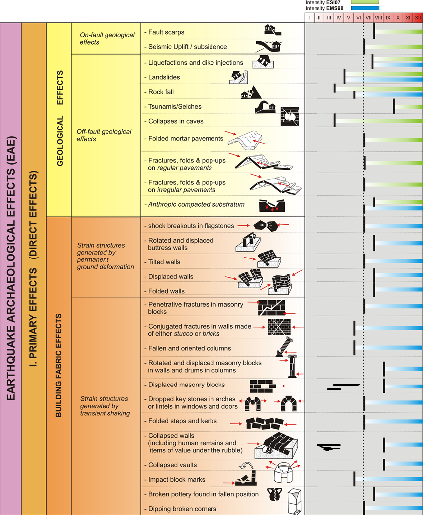 Earthquake Archeological
Effects Chart
Earthquake Archeological
Effects Chart
Click on image to open in a new tab
Rodríguez-Pascua et al (2013) - Environmental Effects (ESI 2007)
 Graphic Representation of
ESI 2007 Intensity
Graphic Representation of
ESI 2007 Intensity
Click on image to open in a new tab
- Synoptic Table of ESI 2007
Intensity Degrees from Michetti et al. (2007)
 Synoptic Table of ESI 2007
Intensity Degrees
Synoptic Table of ESI 2007
Intensity Degrees
Accuracy improves in higher degrees, especially VIII–XII.
Click on image to open in a new tab
Michetti et al. (2007) - Environmental Effects vs. Intensity
from Michetti et al. (2007)
 Diagnostic ranges for
environmental effects by intensity
Diagnostic ranges for
environmental effects by intensity
Click on image to open in a new tab
Michetti et al. (2007)

| Effect | Location | Image(s) | Description | Intensity |
|---|---|---|---|---|
|
Trench T1
Fig. 6e
Map of trenches T1 and T3 area detailing the locations of all other features in the figure (panels a-d). click on image to open in a new tab Kanari et al (2020) |
Dewatering Structure
Fig. 6c
Liquefaction features and their spatial extent. T1 liquefaction fluid escape structures (interpreted in yellow on photo) and its charcoal ET02 sample; white arrow points out liquefaction related feature. click on image to open in a new tab Kanari et al (2020) |
|
|
-
PGA Estimation Chart for sand blows
from Obermeier (1996)
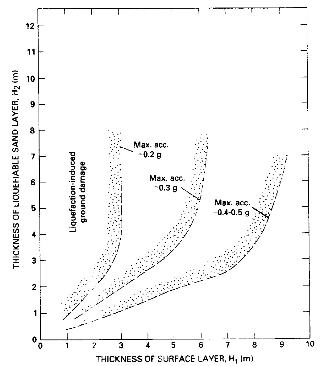 Fig. 9
Proposed boundary curves relating thickness of nonliquefiable surface layer to thickness of the liquefiable zone as a function of peak earthquake accelerations required to induce venting or ground rupturing at the surface
From Ishihara (1985)
click on image t open in a new tab
Obermeier (1996)
| Effect | Location | Image(s) | Description | PGA (g) |
|---|---|---|---|---|
|
Trench T3
Fig. 6e
Map of trenches T1 and T3 area detailing the locations of all other features in the figure (panels a-d). click on image to open in a new tab Kanari et al (2020) |
Sand Blow SB1
Fig. 6a
Liquefaction features and their spatial extent. Trench log of Sand blow 1 structure (SB1) in T3 and its logged stratigraphic structure; boundaries of sand blow outlined in black dashed rectangle; L1-L7 are stratigraphic units of the West Sabkha (see text for detail). Yellow hexagons mark charcoal samples locations; dated samples have adjacent radiocarbon age determinations presented click on image to open in a new tab Kanari et al (2020) Sand Blow SB2
Fig. 6b
Liquefaction features and their spatial extent. photo mosaic of Sand blow 2 structure (SB2) in T3; no detailed log is available for SB2 click on image to open in a new tab Kanari et al (2020) |
|
|
Source - Wells and Coppersmith (1994)
| Variable | Input | Units | Notes |
|---|---|---|---|
| cm. | |||
| cm. | |||
| m/s | Enter a value of 655 for no site effect Equation comes from Darvasi and Agnon (2019) |
||
| Variable | Output - not considering a Site Effect | Units | Notes |
| unitless | Moment Magnitude for Avg. Displacement | ||
| unitless | Moment Magnitude for Max. Displacement | ||
| Variable | Output - Site Effect Removal | Units | Notes |
| unitless | Reduce Intensity Estimate by this amount to get a pre-amplification value of Intensity |
The value given for Intensity with site effect removed is how much you should subtract from your Intensity estimate to obtain a pre-amplification value for Intensity. For example if the output is 0.5 and you estimated an Intensity of 8, your pre-amplification Intensity is now 7.5. An Intensity estimate with the site effect removed is helpful in producing an Intensity Map that will do a better job of "triangulating" the epicentral area. If you enter a VS30 greater than 655 m/s you will get a positive number, indicating that the site amplifies seismic energy. If you enter a VS30 less than 655 m/s you will get a negative number, indicating that the site attenuates seismic energy rather than amplifying it. Intensity Reduction (Ireduction) is calculated based on Equation 6 from Darvasi and Agnon (2019).
VS30 is the average seismic shear-wave velocity from the surface to a depth of 30 meters at earthquake frequencies (below ~5 Hz.). Darvasi and Agnon (2019) estimated VS30 for a number of sites in Israel. If you get VS30 from a well log, you will need to correct for intrinsic dispersion. There is a seperate geometric dispersion correction usually applied when processing the waveforms however geometric dispersion corrections are typically applied to a borehole Flexural mode generated from a Dipole source and for Dipole sources propagating in the first 30 meters of soft sediments, modal composition is typically dominated by the Stoneley wave. Shear from Stoneley estimates are approximate at best. This is a subject not well understood and widely ignored by the Geotechnical community and/or Civil Engineers but understood by a few specialists in borehole acoustics. Other considerations will apply if you get VS30 value from a cross well survey or a shallow seismic survey where the primary consideration is converting shear slowness from survey frequency to Earthquake frequency. There are also ways to estimate shear slowness from SPT & CPT tests.
Fig. 9
Proposed boundary curves relating thickness of nonliquefiable surface layer to thickness of the liquefiable zone as a function of peak earthquake accelerations required to induce venting or ground rupturing at the surface
From Ishihara (1985)
click on image t open in a new tab
Obermeier (1996)
| Sand Blow | Sand Blow Thickness (m) | Thickness of Surface Layer (m) |
|---|---|---|
| SB1 | 1 | ? |
| SB2 | 1 | ? |
| Variable | Input | Units | Notes |
|---|---|---|---|
| g | Peak Horizontal Ground Acceleration | ||
| Variable | Output (No Site Effect) |
Units | Notes |
| unitless | Conversion from PGA to Intensity using Wald et al (1999) |
Abueladas, A.-R., et al. (2020). Liquefaction susceptibility maps for the Aqaba-Elat region with projections of future hazards with sea level rise, Quarterly Journal of Engineering Geology and Hydrogeology 54: qjegh2020-2039.
Ash-Mor, A., et al. (2017). Micropaleontological and taphonomic characteristics of mass transport deposits in the northern Gulf of Eilat/Aqaba, Red Sea, Marine Geology 391.
Kanari, M., et al. (2015). On-land and offshore evidence for Holocene earthquakes in the Northern Gulf of Aqaba-Elat, Israel/Jordan, Miscellanea INGV 27: 240–243.
Kanari, M., et al. (2020). Seismic potential of the Dead Sea Fault in the northern Gulf of Aqaba-Elat: new evidence from liquefaction, seismic reflection, and paleoseismic data
, Tectonophysics 793: 228596.