Map Info
DEMs
Topography
Bathymetry
Mapping software
ESRI
Coding
Cartography
Magnetic Calculator
Drones
Photogrammetry
Lidar
GPS
Geographic Data
Spatial Statistics
Epicenter Location
Several site-attributes are considered:
- Construction quality – Equal ground acceleration will cause different damage to manmade structures depending on their material and construction (Bolt, 1978). In general, the quality of construction at the beginning of the 20th century is considered to be low and this is well described by Michaeli (1928) and Willis (1928), both experts that advised the government of necessary repairs after the earthquake. However, one could distinguish between two levels of construction quality. Towards the end of the 19th century, massive growth in Jewish population (Ben-Arieh, 1981) resulted establishments of new settlements (e.g., Tel Aviv, Petah Tiqwa) or expansion of existing such as Jerusalem and Haifa. These were built with contemporaneous new techniques and materials such as iron casting, cement and concrete (Fuchs, 1998; Krivoruchko, 1996) while Arabic settlements were less developed and were based primary upon pre 20th century traditional construction techniques, considered to be less resistant to shaking because of extensive use of raw materials such as adobe and wood. Accordingly, we classify localities into two groups of construction quality in which the Jewish settlements are considered stable (Table 1) and thus, ascribe exaggeration of intensities to the Arabic settlements.
- Topographic slope – the relation between damage and the underlying topographic slope is found to be significant (e.g., Athanasopoulos et al., 1988; Avni, 1999; Evernden et al., 1973; Wust-Bloch, 2002; Zaslavsky et al., 2000). Moreover, the larger the ratio between the height of the mountain peak above its surroundings to its width, the higher is the amplification (Salamon et al., 2010). Slope was calculated using a digital elevation model (DEM) of Hall and Cleave (1998) attributed with resolution of 25 m per pixel along with horizontal and vertical errors ranging between 10–50 m and less than 10 m for 95% of the data respectively. Because the resolution is too low to use this DEM for calculating topographic slopes of individual structures, the slope of the area of each locality is calculated. Having a max slope value of 31°, we decided to use the median (15°) as a threshold of steep slope in which localities attributed with slope greater than this threshold are presumed to be overestimated (Table 1).
- Groundwater level depth – P and S waves behave differently as they pass through solid and liquid volumes. P waves travel trough both volumes, while the S waves travel only through solid and tends to be absorbed in liquid (Bolt, 1978; Evernden et al., 1973). Researchers (e.g., Yang and Sato, 2000) found that depth of underground groundwater level, mainly in the manner of saturation and thickness, affects the movement of the ground in soft soils such as alluvial areas. Full analysis of this issue is rather complex and beyond the scope of our paper. Yet, we examine the groundwater level depth as a possible influencing factor. This is held using data of drills and boreholes collected in 1933/4 during a comprehensive survey throughout mandatory Palestine (Blake and Goldschmidt, 1947). Comparison of precipitation recorded in 1927 and 1933/4 enables to trace the fluctuation of groundwater level depth of the two sequences and estimate their 1927 contemporaneous depth. Nevertheless, accuracy of the data is limited and fraught with uncertainties whereas many of the localities are attributed with interpolated-based values. Furthermore, the 1933–4 groundwater level could have been influenced by the earthquake itself. Consequently, only intensity in localities with very shallow groundwater depth i.e., between 0 and 10 m (Table 1), were considered to be amplified.
- Surface geology – amplification occurs when there is a
considerable decrease in shear wave velocity (Vs) toward the surface
layers. Localities built on unconsolidated soils are likely to
suffer more damage than those built on rocks (Yeats et al., 1997).
Accordingly, we categorized localities into three surface
geology classes (Table 1):
- unconsolidated soil
- soft rock (clay and marlstone)
- solid rock
which tend to attenuate damage and thus, lead to underestimation of intensity. - Population – Ambraseys (1971) found a correlation between density of populations to post-earthquake reports in which reports of densely populated area tend to be exaggerated. Feldman and Shapira (1994) found a tendency for higher estimation of seismic intensity in large cities such as Jerusalem and Tel Aviv. Consequently, we categorize localities into two classes defined by a population threshold of 5000 residents (Table 1)
To determine which of the site-attributes is significant, a multi- linear regression is carried out:
Y = α1*X1 + α2*X2 + ... αn*Xn + β (1)
Whereas Y is the mode intensity of a given locality, X1-n represents a given site-attribute and α, β are the regression's slope and intercept respectively.
The significance of each site-attribute's correlation with intensity is listed in Table 1. Besides population, the correlation of all other four site-attributes with the intensity is found to be significant, meaning that we can reject the null hypothesis of no impact over the intensity. Accordingly, the population site-attribute was excluded from of the correction procedure.
Correction rate was set to the standard error of the mode intensity of (Avni, 1999). Being almost identical to one MSK unit (STD=1.2419), the correction rate was refined accordingly to a value of 1 (Table 1)and is based upon linearity assumption that is, the difference between intensity 3 and 4 is identical as between 8 and 9. Out of 133 inspected localities, 111 were corrected.
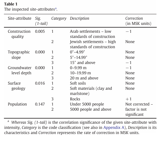 Table 1
The inspected site-attributes
Zohar and Marco (2012)

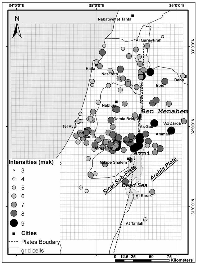
The study area at the central Dead Sea Transform (DST) and suspected active faults (after Bartov et al., 2002). The map contains two previously suggested epicenters of the 6.25 ML 1927 Jericho earthquake (marked in black asterisks):
- Ben Menahem et al. (1976)
- Avni (1999) and Avni et al. (2002)
Fig. 2 (middle)
The research area with depiction of
- Spatial distribution of mode intensities evaluated by Avni, 1999, ranging from 3 to 9 in the MSK scale
- 5*5 km grid-cell structure representing 2501 assumed epicenters to be validated with the intensity data
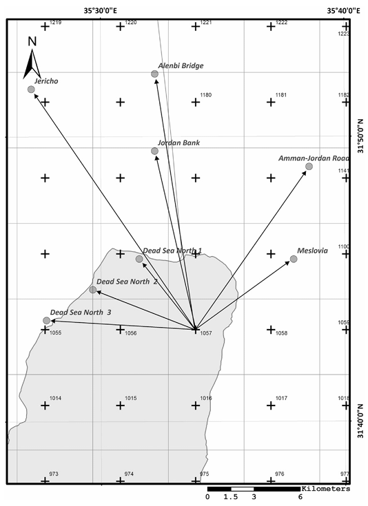
Fig. 3 (right)
Illustration of epicentral distances calculation for grid cell (assumed epicenter) 1057 to its surrounding intensities
all Figures from Zohar and Marco (2012)
Most of the seismic activity in the area is related to the Dead Sea Transform (DST) (Garfunkel et al., 1981). Thus, our inspected geographic area covers the central of DST region extending between 33.96˚ to 36.06˚ and 30.94˚ to 33.26˚ in the east–west and south–north axis respectively (Fig. 1). Initially, a set of assumed epicenters is generated and arranged in a 5*5 km grid-cell structure in which each polygon cell represents an assumed epicenter, totaling 2501 inspected cells (Fig. 2). Then we iterate these cells and calculate epicentral distances to the intensity localities (Fig. 3). However, the decay of intensity with distance is non linear and depends also on the azimuthal variations of the radiated energy (Howell and Schulz, 1975), anisotropic wave propagations (Stromeyer and Grunthal, 2009) and local site-effects (Bolt, 1978). Therefore, logarithmic proportionality (e.g., Bakun, 2006; Bakun and Scotti, 2006; Howell and Schulz, 1975; Stromeyer and Grunthal, 2009) is commonly used to describe this relationship. Following this approach, we adopt the attenuation relation developed by Stromeyer and Grunthal (2009) after Sponheuer (1960):
I = I* - a*log(SQRT[(R2+h2)/h2]) -b*[SQRT(R2+h2)-h] (2)
Where I is the given intensity, I* is an estimate of the I0 (Pasolini et al., 2008), a and b are constants representing the geometric spreading and absorption of energy respectively, R is the epicentral distance and h is the rupture depth. Assuming that I*, a and b are constants, I depends on the following logarithmic proportionality:
I = log(SQRT[(R2+h2)/h2]) - [SQRT(R2+h2)-h] (3)
Taking into consideration that most earthquakes that are related to the DST are generated in depth of up to 15 km (Shapira, 1979), h was set to 15 km and accordingly, a logarithmic factor for each of the epicentral distances calculated previously was generated.
Finally, for each cell we have correlated the intensities and their adjacent logarithmic factor of distance and use the ‘Pearson’ estimate as a quality indicator.
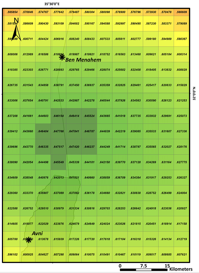
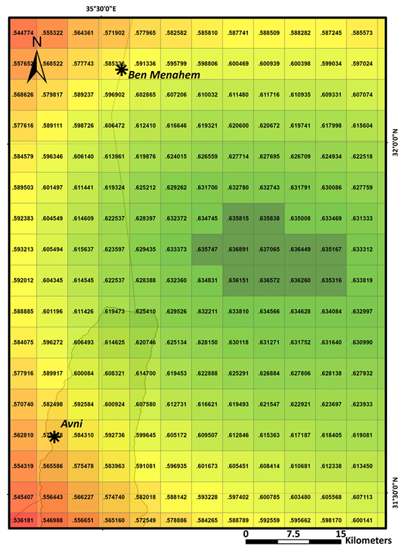
Pearson correlation values of grid cells (assumed epicenters) correlated with corrected intensity data. Low values are colored in light red while high values are represented by dark green colors. A cluster of the highest values at the center of the figure represents the model preferred epicenter located between the two previously suggested epicenters of Avni et al. (2002) and Ben Menahem et al. (1976) (marked in black asterisks).
Fig. 5 (middle)
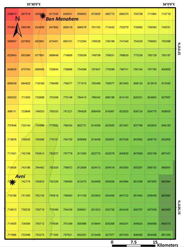
Pearson correlation values of grid cells (assumed epicenters) correlated with raw intensity data that was not corrected. Low values are colored in light red while high values are represented by dark green colors. A cluster of the highest values is emphasized at the right edge of the figure representing the model suggestion for the epicenter. This location is some 25 km east of the DST region and is less consistent with the two previously suggested of Avni et al. (2002) and Ben Menahem et al. (1976) (marked in black asterisks).
Fig. 6 (right)
Pearson correlation values of grid cells (assumed epicenters) correlated with exaggerated corrected intensity data. Low values are colored in light red while high values are represented by dark green colors. A cluster of the highest values is emphasized at the right edge of the figure representing the model suggestion for the epicenter. This location is some 60 km east of the DST region and by far distant from the two previously suggested epicenters of Avni et al. (2002) and Ben Menahem et al. (1976) (marked in black asterisks).
All Figures from Zohar and Marco (2012)
Upon completeness of all 2501 cell correlations, we scaled and examined their Pearson indicators. These values range between 0.2061 and 0.6478 whereas the highest values are related to cells located at the north of the Dead Sea. Fig. 4 demonstrates a graduated colored grid in which each of its cells represents an adjacent Pearson indicator of an assumed epicenter. The highest correlation values, covering an area of approximately 50 km2 , are emphasized indicating the statistically most appropriate location of the epicenter. The center of mass of this area is located within the DST region and is about 35 km north of the epicenter calculated by Avni et al. (2002) and ~25 km south of the one calculated by Ben Menahem et al. (1976). Considering that the expected subsurface rupture length of such magnitude is approximately 20 km (Wells and Coppersmith, 1994), we conclude that this model is consistent with previous suggested locations with possible error of up to 50 km.
To demonstrate the importance of intensity correction we implement a similar model only with intensity data that was not corrected i.e., the raw mode intensity of Avni (1999). The result of this model is presented in Fig. 5 in which the suggested location is some 25 km east of the DST region. Furthermore, this indication is nearly 45 km northeast to Avni's calculation and 35 south-east of Ben-Menahem. That is, correction of the intensity yields a location that is more consistent with previous calculations than using uncorrected data.
Sensitivity of the model is also to be tested. This is done using exaggerated correction rate i.e., correcting the intensity with 2 MSK units instead of 1. The results are shown in Fig. 6 and demonstrate a location which is distant by far from the DST and the two previous calculations.
- Fig. 1 Location Map
from Zohar and Marco (2012)
Fig. 1
The study area at the central Dead Sea Transform (DST) and suspected active faults (after Bartov et al., 2002). The map contains two previously suggested epicenters of the 6.25 ML 1927 Jericho earthquake (marked in black asterisks):
- Ben Menahem et al. (1976)
- Avni (1999) and Avni et al. (2002)
Zohar and Marco (2012) - Fig. 2 Intensity
Distribution Map from Zohar and Marco (2012)
Fig. 2
The research area with depiction of
- Spatial distribution of mode intensities evaluated by Avni, 1999, ranging from 3 to 9 in the MSK scale
- 5*5 km grid-cell structure representing 2501 assumed epicenters to be validated with the intensity data
Zohar and Marco (2012) - Fig. 3 Illustration
of epicentral distances calculation for grid cell from Zohar and Marco (2012)
Fig. 3
Illustration of epicentral distances calculation for grid cell (assumed epicenter) 1057 to its surrounding intensities
Zohar and Marco (2012) - Fig. 4 Pearson
correlation values of grid cells (assumed epicenters) correlated with corrected intensity data from Zohar and Marco (2012)
Fig. 4
Pearson correlation values of grid cells (assumed epicenters) correlated with corrected intensity data. Low values are colored in light red while high values are represented by dark green colors. A cluster of the highest values at the center of the figure represents the model preferred epicenter located between the two previously suggested epicenters of Avni et al. (2002) and Ben Menahem et al. (1976) (marked in black asterisks).
Zohar and Marco (2012) - Fig. 5 Pearson
correlation values of grid cells (assumed epicenters) correlated with raw uncorrected intensity data from Zohar and Marco (2012)
Fig. 5
Pearson correlation values of grid cells (assumed epicenters) correlated with raw intensity data that was not corrected. Low values are colored in light red while high values are represented by dark green colors. A cluster of the highest values is emphasized at the right edge of the figure representing the model suggestion for the epicenter. This location is some 25km east of the DST region and is less consistent with the two previously suggested of Avni et al. (2002) and Ben Menahem et al. (1976) (marked in black asterisks).
Zohar and Marco (2012) - Fig. 6 Pearson
correlation values of grid cells (assumed epicenters) correlated with exaggerated corrected intensity data from Zohar and Marco (2012)
Fig. 6
Pearson correlation values of grid cells (assumed epicenters) correlated with exaggerated corrected intensity data. Low values are colored in light red while high values are represented by dark green colors. A cluster of the highest values is emphasized at the right edge of the figure representing the model suggestion for the epicenter. This location is some 60 km east of the DST region and by far distant from the two previously suggested epicenters of Avni et al. (2002) and Ben Menahem et al. (1976) (marked in black asterisks).
Zohar and Marco (2012)
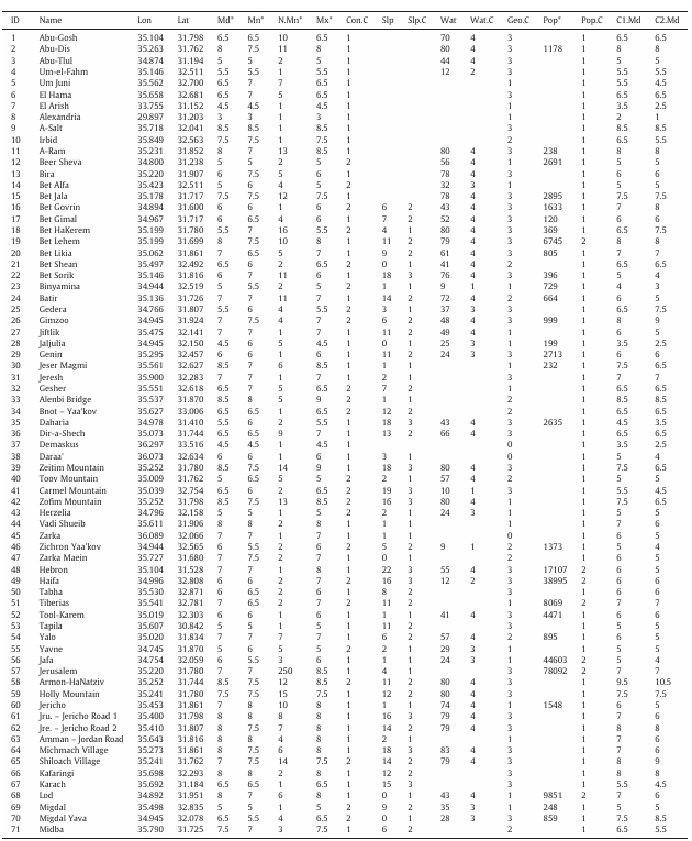
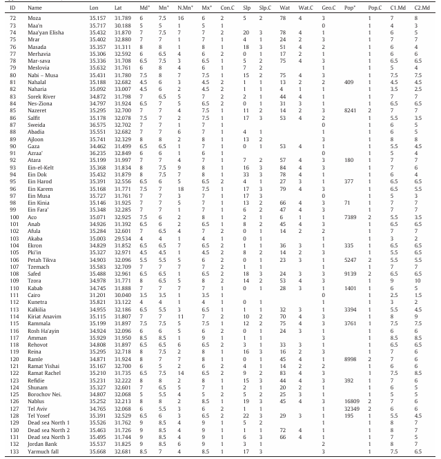
Database of the research
Description of fields and their adjacent abbreviations (in brackets):
- Sequential id of localities (ID)
- locality name (Name)
- Longitude in Decimal Degrees (Lon)
- Latitude Decimal Degrees (Lat)
- Mode intensity (Md)
- Mean intensity (Mn)
- Number of observations for mean intensity (N.Mn)
- Max intensity (Mx)
- Construction quality category (Con.C)
- Slope (in degrees) (Slp)
- Slope category (Slp.C)
- Groundwater level (in meters)(Wat)
- Groundwater level category (Wat.C)
- Surface geology category (Geo.C)
- Population(Pop)
- Population category(Pop.C)
- Corrected mode intensity using a rate of 1 MSK unit (C1.Md)
- Corrected mode intensity using a rate of 2 MSK units (C2.Md)
* fields 5–8 contain raw intensity data and field 15 contain the 1927 population following Avni (1999)
Zohar and Marco (2012)