
SEISCALC
Earthquake Science Calculators
Coded by Jefferson Williams
Caveat: For use in Historical Earthquake Research - not for Engineering work.
Seismic Attenuation
Magnitude Estimation (Scaling Relationships)

Figure 2
Map of the broader Aegean Region showing the distribution of all the morphogenic earthquakes (sensu Caputo, 1993) and corresponding co-seismic ruptures considered in the present research. Numbers refer to the year of the seismic event; the bars are oriented parallel to the fault traces, while the length of the bars is roughly proportional to SRL. Data from Table 2
Pavlides and Caputo (2004)
Pavlides and Caputo (2004) examined a dataset of earthquakes from the
broader Aegean Region(see Fig. 2 above) and developed a series of empirically based equations to estimate surface magnitude (MS) of an earthquake from local observations of surface rupture length (SRL), maximum vertical displacement (MVD), and/or average displacement (AD). This resulted in the following regression equations:
MS = 0.90*log10(SRL) + 5.48 Equation 1
MS = 0.59*log10(MVD) + 6.75 Equation 2
These equations showed good correlation coefficients (0.84 and 0.82 respectively). Pavlides and Caputo (2004:1) noted that
co-seismic fault rupture lengths and especially maximum displacements in the Aegean Region have systematically lower values than the same parameters worldwide, but are similar to those of the Eastern Mediterranean–Middle East region. Pavlides and Caputo (2004) also developed equations to estimate the max and min surface magnitude (MS) from local observations of surface rupture length (SRL), maximum vertical displacement (MVD), and/or average displacement (AD). These are shown below:
MSmax = 1.00*log10(SRL) + 5.60 Equation 5
MSmax = 0.48*log10(MVD) + 7.04 Equation 6
MSmin = 1.42*log10(SRL) + 4.36 Equation 7
MSmin = 0.87*log10(MVD) + 6.53 Equation 8
Pavlides and Caputo (2004) also presented equations to solve for surface rupture length (SRL) and maximum vertical displacement (MVD) from surface magnitude (MS):
log10(SRL) = 0.78*MS - 3.93 Equation 3
log10(MVD) = 1.14*MS - 7.82 Equation 4
Figures 5 and 6 (below) show differences between the equations of Wells and Coppersmith (1994), Ambraseys and Jackson (1998), Pavlides and Caputo (2004), and Papazachos and Papazachou (1989).
 Figure 5
Comparison between regression curves for Ms versus SRL, proposed by Wells and Coppersmith (1994) for normal faulting from worldwide data (W&C’94) and by Ambraseys and Jackson (1998) for the Mediterranean region (A&J’98). The curve from Papazachos and Papazachou (1989) has been recalculated according to their data because of a typographic error in the given equations (P&P’89). The best-fit regression curve as well as the upper and lower envelopes based on this research is also represented.
Pavlides and Caputo (2004)
 Figure 6
Comparison between regression curves for Ms versus MVD, proposed by Wells and Coppersmith (1994) for normal faulting from worldwide data (W&C’94) and by Ambraseys and Jackson (1998) for the Mediterranean region (A&J’98). The curve from Papazachos and Papazachou (1989) has been recalculated according to their data because of a typographic error in the given equations (P&P’89). The best-fit regression curve as well as the upper and lower envelopes based on this research is also represented.
Pavlides and Caputo (2004)
- from Wells and Coppersmith (1994)
- Fig. 11 Regression of average
surface displacement on magnitude from Wells and Coppersmith (1994)
 Fig. 11
- Regression of average surface displacement on magnitude (M). Regression line shown for all-slip-type relationship. Short dashed line indicates 95% confidence interval.
- Regression lines for strike-slip, reverse, and normal-slip relationships.
See Table 2 for regression coefficients. Length of regression lines shows the range of data for each relationship.
click on image to open in a new tab
Wells and Coppersmith (1994) - Fig. 10 Regression of maximum
surface displacement on magnitude from Wells and Coppersmith (1994)
 Fig. 10
- Regression of maximum surface displacement on magnitude (M). Regression line shown for all-slip-type relationship. Short dashed line indicates 95% confidence interval.
- Regression lines for strike-slip, reverse, and normal-slip relationships.
See Table 2 for regression coefficients. Length of regression lines shows the range of data for each relationship.
click on image to open in a new tab
Wells and Coppersmith (1994) - Fig. 13 Surface rupture length
on average displacement from Wells and Coppersmith (1994)
 Fig. 13
- Regression of surface rupture length on average displacement. Regression line shown for all-slip-type relationship. Short dashed line indicates 95% confidence interval.
- Regression lines for strike-slip, reverse, and normal-slip relationships.
See Table 2 for regression coefficients. Length of regression lines shows the range of data for each relationship.
click on image to open in a new tab
Wells and Coppersmith (1994) - Fig. 12 Surface rupture length
on maximum displacement from Wells and Coppersmith (1994)
 Fig. 12
- Regression of surface rupture length on maximum displacement. Regression line shown for all-slip-type relationship. Short dashed line indicates 95% confidence interval.
- Regression lines for strike-slip, reverse, and normal-slip relationships.
See Table 2 for regression coefficients. Length of regression lines shows the range of data for each relationship.
click on image to open in a new tab
Wells and Coppersmith (1994) - Fig. 14 Regression of subsurface
rupture length on magnitude from Wells and Coppersmith (1994)
 Fig. 14
- Regression of subsurface rupture length on magnitude (M). Regression line shown for all-slip-type relationship. Short dashed line indicates 95% confidence interval.
- Regression lines for strike-slip relationships.
See Table 2 for regression coefficients. Length of regression lines shows the range of data for each relationship.
click on image to open in a new tab
Wells and Coppersmith (1994) - Table 2A Regressions of Rupture Length,
Rupture Width, Rupture Area, and Moment Magnitude from Wells and Coppersmith (1994)
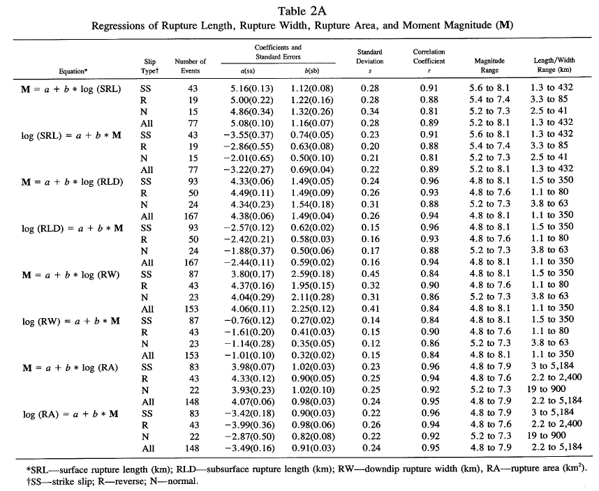 Table 2A
Regressions of Rupture Length, Rupture Width, Rupture Area, and Moment Magnitude (M)
click on image to open in a new tab
Wells and Coppersmith (1994) - Table 2B Regression of displacement
and moment magnitude from Wells and Coppersmith (1994)
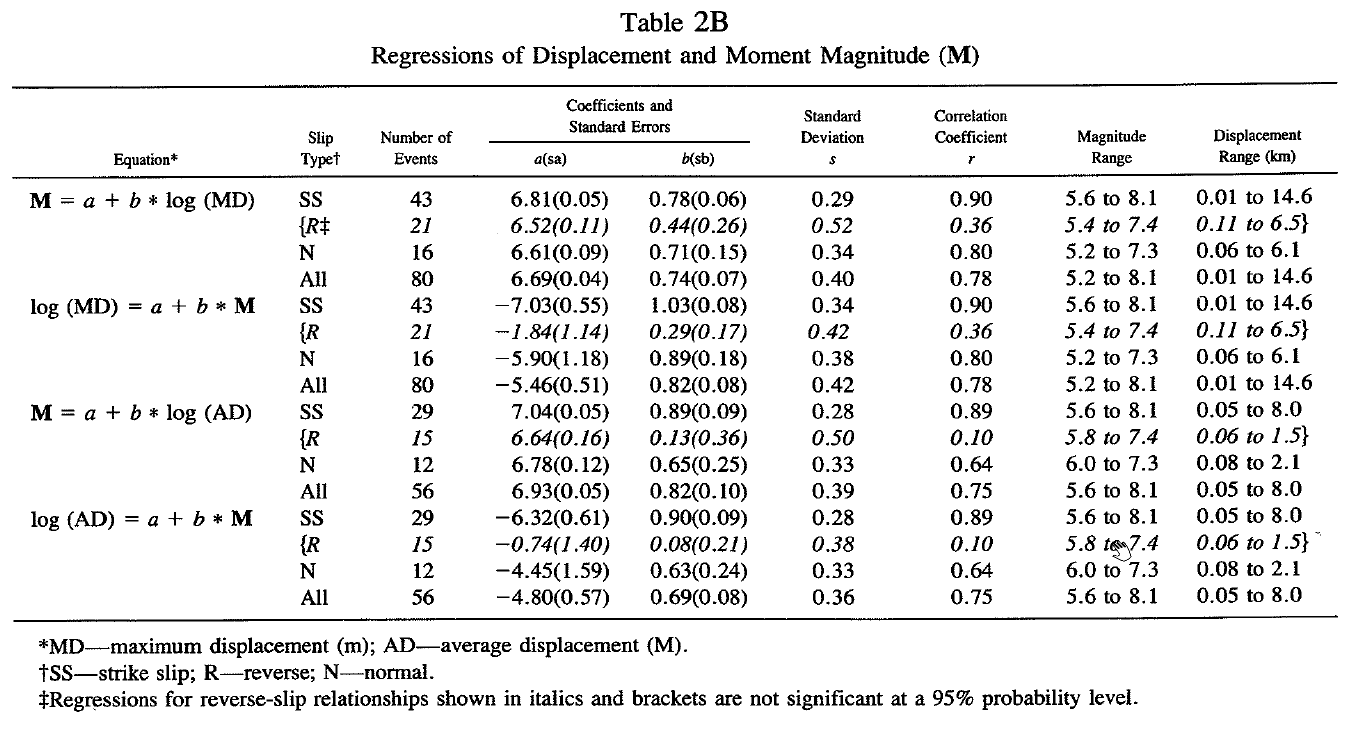 Table 2B
Regressions of displacement and moment magnitude (M).
click on image to open in a new tab
Wells and Coppersmith (1994) - Table 2C Regression of surface
rupture length and displacement from Wells and Coppersmith (1994)
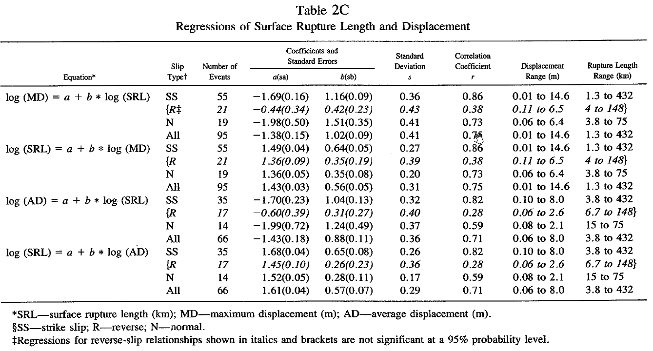 Table 2C
Regressions of surface rupture length and displacement.
click on image to open in a new tab
Wells and Coppersmith (1994)
| Variable | Input | Units | Notes | ||
|---|---|---|---|---|---|
| cm. | Strike-Slip displacement | ||||
| cm. | Strike-Slip displacement | ||||
| Variable | Output - not considering a Site Effect | Units | Notes | ||
| unitless | Moment Magnitude for Avg. Displacement (Table 2B, SS) | ||||
| unitless | Moment Magnitude for Max. Displacement (Table 2B, SS) | ||||
| SRL from Avg. Displacement | Direct km | Plotted km | km | Surface Rupture Length, Table 2C SS — hover Direct/Plotted for equations | |
| SRL from Max. Displacement | Direct km | Plotted km | km | Surface Rupture Length, Table 2C SS — hover Direct/Plotted for equations | |
| RLD from Avg. Displacement | Direct1 km | Direct2 km | Plotted km | km | Subsurface Rupture Length, Table 2A SS (via Mw) — hover Direct1/Direct2/Plotted for equations |
| RLD from Max. Displacement | Direct1 km | Direct2 km | Plotted km | km | Subsurface Rupture Length, Table 2A SS (via Mw) — hover Direct1/Direct2/Plotted for equations |
- All curves are strike-slip (SS) regressions from Wells and Coppersmith (1994), plotted over a fixed range of 1-1000 cm displacement on a log x-axis; markers overlay the current Average and Maximum Displacement inputs above. Curves/markers are colored by method: Direct1 in blue (RLD plot only), Direct / Direct2 in green, Plotted in purple — solid (SRL plot) or dot (RLD plot) for the Average-Displacement relation, dashed for the Maximum-Displacement relation.
- MW vs. Displacement (Table 2B, SS): MW = 7.04 + 0.89·log10(Avg. Displacement) and MW = 6.81 + 0.78·log10(Max. Displacement), displacement in meters.
- Surface Rupture Length (SRL): Table 2C provides a genuine second, independently-fit source that skips Mw entirely, so Direct and Plotted are two different lines. Direct (Table 2C's own fit in the needed direction): SRL = 10(1.68 + 0.65·log10(Avg. Displacement in m)) km, SRL = 10(1.49 + 0.64·log10(Max. Displacement in m)) km. Plotted (algebraic inversion of Table 2C's forward fit, matches Figs. 12/13 exactly): SRL = 10(1.6346 + 0.9615·log10(Avg. Displacement in m)) km, SRL = 10(1.4569 + 0.8621·log10(Max. Displacement in m)) km — derived by solving log10(AD) = -1.70 + 1.04·log10(SRL) and log10(MD) = -1.69 + 1.16·log10(SRL) (Table 2C SS, the actual "Strike Slip" lines drawn in Figs. 13 and 12) for log10(SRL). These two differ because ordinary least-squares regression is direction-dependent: Table 2C's own SRL-from-displacement row minimizes error in the log(SRL) direction, while its displacement-from-SRL row (used by Plotted) minimizes error in the log(displacement) direction -- two different best-fit lines unless the correlation is perfect.
- Subsurface Rupture Length (RLD): Table 2A relates RLD to magnitude, not displacement, so all three answers below still go via Mw (the Mw already computed in the cells above) — there remains no Table 2C-style direct RLD-vs-displacement regression to skip that step entirely. However, Table 2A actually publishes regressions in both directions for the RLD-magnitude relationship (as Table 2B and Table 2C do for their own relationships), so RLD now gets three answers instead of two: Direct1 uses Table 2A's own reverse-direction fit, strike-slip, directly (no inversion): log10(RLD) = -2.57 + 0.62·MW, i.e. RLD = 10(-2.57 + 0.62·MW) km. Direct2 is the algebraic inversion of Table 2A's forward fit relating magnitude to RLD (strike-slip): M = 4.33 + 1.49·log10(RLD), which solves to RLD = 10(-2.9060 + 0.6711·MW) km — this was the only "Direct" answer this calculator gave before Direct1 was added. Plotted reads the same equation as Direct2 off the exact "Strike Slip" line WC94 drew in Fig. 14 (M vs. RLD), so Direct2 and Plotted necessarily coincide and read the same values, exactly as before. Direct1 is the genuinely independent one: because it comes from Table 2A's separate reverse-direction row rather than an inversion of the forward row, it will generally give a different RLD than Direct2/Plotted — mirroring how Table 2C's Direct differs from its Plotted for SRL.
- ⚠️ Range warning: each output cell now checks its governing input (or, for RLD, the Mw value it depends on) against the exact Magnitude/Displacement/ Rupture-Length Range columns published for the strike-slip rows of Tables 2A, 2B, and 2C. An orange ⚠️ tag appears next to a value whenever the calculation is extrapolating beyond the range of data Wells and Coppersmith actually regressed — hover it for the exact valid range. This is a warning only; it never changes, clamps, or blocks a computed result.
- from Wells and Coppersmith (1994)
- Fig. 11 Regression of average
surface displacement on magnitude from Wells and Coppersmith (1994)
Fig. 11
- Regression of average surface displacement on magnitude (M). Regression line shown for all-slip-type relationship. Short dashed line indicates 95% confidence interval.
- Regression lines for strike-slip, reverse, and normal-slip relationships.
See Table 2 for regression coefficients. Length of regression lines shows the range of data for each relationship.
click on image to open in a new tab
Wells and Coppersmith (1994) - Fig. 10 Regression of maximum
surface displacement on magnitude from Wells and Coppersmith (1994)
Fig. 10
- Regression of maximum surface displacement on magnitude (M). Regression line shown for all-slip-type relationship. Short dashed line indicates 95% confidence interval.
- Regression lines for strike-slip, reverse, and normal-slip relationships.
See Table 2 for regression coefficients. Length of regression lines shows the range of data for each relationship.
click on image to open in a new tab
Wells and Coppersmith (1994) - Fig. 13 Surface rupture length
on average displacement from Wells and Coppersmith (1994)
Fig. 13
- Regression of surface rupture length on average displacement. Regression line shown for all-slip-type relationship. Short dashed line indicates 95% confidence interval.
- Regression lines for strike-slip, reverse, and normal-slip relationships.
See Table 2 for regression coefficients. Length of regression lines shows the range of data for each relationship.
click on image to open in a new tab
Wells and Coppersmith (1994) - Fig. 12 Surface rupture length
on maximum displacement from Wells and Coppersmith (1994)
Fig. 12
- Regression of surface rupture length on maximum displacement. Regression line shown for all-slip-type relationship. Short dashed line indicates 95% confidence interval.
- Regression lines for strike-slip, reverse, and normal-slip relationships.
See Table 2 for regression coefficients. Length of regression lines shows the range of data for each relationship.
click on image to open in a new tab
Wells and Coppersmith (1994) - Fig. 14 Regression of subsurface
rupture length on magnitude from Wells and Coppersmith (1994)
Fig. 14
- Regression of subsurface rupture length on magnitude (M). Regression line shown for all-slip-type relationship. Short dashed line indicates 95% confidence interval.
- Regression lines for strike-slip relationships.
See Table 2 for regression coefficients. Length of regression lines shows the range of data for each relationship.
click on image to open in a new tab
Wells and Coppersmith (1994) - Table 2A Regressions of Rupture Length,
Rupture Width, Rupture Area, and Moment Magnitude from Wells and Coppersmith (1994)
Table 2A
Regressions of Rupture Length, Rupture Width, Rupture Area, and Moment Magnitude (M)
click on image to open in a new tab
Wells and Coppersmith (1994) - Table 2B Regression of displacement
and moment magnitude from Wells and Coppersmith (1994)
Table 2B
Regressions of displacement and moment magnitude (M).
click on image to open in a new tab
Wells and Coppersmith (1994) - Table 2C Regression of surface
rupture length and displacement from Wells and Coppersmith (1994)
Table 2C
Regressions of surface rupture length and displacement.
click on image to open in a new tab
Wells and Coppersmith (1994)
| Variable | Input | Units | Notes | ||
|---|---|---|---|---|---|
| cm. | Normal-Slip displacement | ||||
| cm. | Normal-Slip displacement | ||||
| Variable | Output - not considering a Site Effect | Units | Notes | ||
| unitless | Moment Magnitude for Avg. Displacement (Table 2B, N) | ||||
| unitless | Moment Magnitude for Max. Displacement (Table 2B, N) | ||||
| SRL from Avg. Displacement | Direct km | Plotted km | km | Surface Rupture Length, Table 2C N — hover Direct/Plotted for equations | |
| SRL from Max. Displacement | Direct km | Plotted km | km | Surface Rupture Length, Table 2C N — hover Direct/Plotted for equations | |
| RLD from Avg. Displacement | Direct1 km | Direct2 km | Plotted km | km | Subsurface Rupture Length, Table 2A N (via Mw) — hover Direct1/Direct2/Plotted for equations |
| RLD from Max. Displacement | Direct1 km | Direct2 km | Plotted km | km | Subsurface Rupture Length, Table 2A N (via Mw) — hover Direct1/Direct2/Plotted for equations |
- All curves are normal-slip (N) regressions from Wells and Coppersmith (1994), plotted over a fixed range of 1-1000 cm displacement on a log x-axis; markers overlay the current Average and Maximum Displacement inputs above. Curves/markers are colored by method: Direct1 in blue (RLD plot only), Direct / Direct2 in green, Plotted in purple — solid (SRL plot) or dot (RLD plot) for the Average-Displacement relation, dashed for the Maximum-Displacement relation.
- MW vs. Displacement (Table 2B, N): MW = 6.78 + 0.65·log10(Avg. Displacement) and MW = 6.61 + 0.71·log10(Max. Displacement), displacement in meters. Unlike Reverse, both normal-slip relationships are statistically significant at 95% confidence per Wells and Coppersmith's own t-tests (r = 0.64 and 0.80).
- Surface Rupture Length (SRL): Table 2C provides a genuine second, independently-fit source that skips Mw entirely, so Direct and Plotted are two different lines. Direct (Table 2C's own fit in the needed direction): SRL = 10(1.52 + 0.28·log10(Avg. Displacement in m)) km, SRL = 10(1.36 + 0.35·log10(Max. Displacement in m)) km. Plotted (algebraic inversion of Table 2C's forward fit, matches Figs. 12/13 exactly): SRL = 10(1.6048 + 0.8065·log10(Avg. Displacement in m)) km, SRL = 10(1.3113 + 0.6623·log10(Max. Displacement in m)) km — derived by solving log10(AD) = -1.99 + 1.24·log10(SRL) and log10(MD) = -1.98 + 1.51·log10(SRL) (Table 2C N, the actual "Normal" lines drawn in Figs. 13 and 12) for log10(SRL). These two differ because ordinary least-squares regression is direction-dependent: Table 2C's own SRL-from-displacement row minimizes error in the log(SRL) direction, while its displacement-from-SRL row (used by Plotted) minimizes error in the log(displacement) direction -- two different best-fit lines unless the correlation is perfect. Both normal-slip Table 2C relationships are statistically significant at 95% confidence (r = 0.59 to 0.73) — unlike Reverse, whose Table 2C relationships WC94 found not significant.
- Subsurface Rupture Length (RLD): Table 2A relates RLD to magnitude, not displacement, so all three answers below still go via Mw (the Mw already computed in the cells above) — there remains no Table 2C-style direct RLD-vs-displacement regression to skip that step entirely. However, Table 2A actually publishes regressions in both directions for the RLD-magnitude relationship (as Table 2B and Table 2C do for their own relationships), so RLD now gets three answers instead of two: Direct1 uses Table 2A's own reverse-direction fit, normal, directly (no inversion): log10(RLD) = -1.88 + 0.50·MW, i.e. RLD = 10(-1.88 + 0.50·MW) km. Direct2 is the algebraic inversion of Table 2A's forward fit relating magnitude to RLD (normal): M = 4.34 + 1.54·log10(RLD), which solves to RLD = 10(-2.8182 + 0.6494·MW) km — this was the only "Direct" answer this calculator gave before Direct1 was added. Unlike strike-slip, Fig. 14(b) plots ONLY a strike-slip line for RLD vs. magnitude — no normal-slip curve is drawn there at all, so Plotted cannot be "read off the figure" the way it is for SRL or for SS's RLD. Instead Plotted reuses the same equation as Direct2, and the two coincide — but here that is simply because there is no figure to read a distinct line from, not because the table and figure happen to agree (as for SS). Direct1 remains the genuinely independent one regardless: because it comes from Table 2A's separate reverse-direction row rather than an inversion of the forward row, it will generally give a different RLD than Direct2/Plotted — mirroring how Table 2C's Direct differs from its Plotted for SRL.
- ⚠️ Range warning: each output cell checks its governing input (or, for RLD, the Mw value it depends on) against the exact Magnitude/Displacement/ Rupture-Length Range columns published for the normal-slip rows of Tables 2A, 2B, and 2C. An orange ⚠️ tag appears next to a value whenever the calculation is extrapolating beyond the range of data Wells and Coppersmith actually regressed — hover it for the exact valid range. This is a warning only; it never changes, clamps, or blocks a computed result.
- from Wells and Coppersmith (1994)
- Fig. 11 Regression of average
surface displacement on magnitude from Wells and Coppersmith (1994)
Fig. 11
- Regression of average surface displacement on magnitude (M). Regression line shown for all-slip-type relationship. Short dashed line indicates 95% confidence interval.
- Regression lines for strike-slip, reverse, and normal-slip relationships.
See Table 2 for regression coefficients. Length of regression lines shows the range of data for each relationship.
click on image to open in a new tab
Wells and Coppersmith (1994) - Fig. 10 Regression of maximum
surface displacement on magnitude from Wells and Coppersmith (1994)
Fig. 10
- Regression of maximum surface displacement on magnitude (M). Regression line shown for all-slip-type relationship. Short dashed line indicates 95% confidence interval.
- Regression lines for strike-slip, reverse, and normal-slip relationships.
See Table 2 for regression coefficients. Length of regression lines shows the range of data for each relationship.
click on image to open in a new tab
Wells and Coppersmith (1994) - Fig. 13 Surface rupture length
on average displacement from Wells and Coppersmith (1994)
Fig. 13
- Regression of surface rupture length on average displacement. Regression line shown for all-slip-type relationship. Short dashed line indicates 95% confidence interval.
- Regression lines for strike-slip, reverse, and normal-slip relationships.
See Table 2 for regression coefficients. Length of regression lines shows the range of data for each relationship.
click on image to open in a new tab
Wells and Coppersmith (1994) - Fig. 12 Surface rupture length
on maximum displacement from Wells and Coppersmith (1994)
Fig. 12
- Regression of surface rupture length on maximum displacement. Regression line shown for all-slip-type relationship. Short dashed line indicates 95% confidence interval.
- Regression lines for strike-slip, reverse, and normal-slip relationships.
See Table 2 for regression coefficients. Length of regression lines shows the range of data for each relationship.
click on image to open in a new tab
Wells and Coppersmith (1994) - Fig. 14 Regression of subsurface
rupture length on magnitude from Wells and Coppersmith (1994)
Fig. 14
- Regression of subsurface rupture length on magnitude (M). Regression line shown for all-slip-type relationship. Short dashed line indicates 95% confidence interval.
- Regression lines for strike-slip relationships.
See Table 2 for regression coefficients. Length of regression lines shows the range of data for each relationship.
click on image to open in a new tab
Wells and Coppersmith (1994) - Table 2A Regressions of Rupture Length,
Rupture Width, Rupture Area, and Moment Magnitude from Wells and Coppersmith (1994)
Table 2A
Regressions of Rupture Length, Rupture Width, Rupture Area, and Moment Magnitude (M)
click on image to open in a new tab
Wells and Coppersmith (1994) - Table 2B Regression of displacement
and moment magnitude from Wells and Coppersmith (1994)
Table 2B
Regressions of displacement and moment magnitude (M).
click on image to open in a new tab
Wells and Coppersmith (1994) - Table 2C Regression of surface
rupture length and displacement from Wells and Coppersmith (1994)
Table 2C
Regressions of surface rupture length and displacement.
click on image to open in a new tab
Wells and Coppersmith (1994)
| Variable | Input | Units | Notes | |||
|---|---|---|---|---|---|---|
| cm. | Seismic slip on the ramps | |||||
| cm. | Seismic slip on the ramps | |||||
| Variable | Output - not considering a Site Effect | Units | Notes | |||
| MW from Avg. Displacement | R-specific⚠️ | All-slip | unitless | Table 2B — hover R-specific/All-slip for equations and significance | ||
| MW from Max. Displacement | R-specific⚠️ | All-slip | unitless | Table 2B — hover R-specific/All-slip for equations and significance | ||
| SRL from Avg. Displacement | Direct-R⚠️ km | Plotted-R⚠️ km | Direct-All km | Plotted-All km | km | Table 2C — hover Direct/Plotted × R-specific/All-slip for equations |
| SRL from Max. Displacement | Direct-R⚠️ km | Plotted-R⚠️ km | Direct-All km | Plotted-All km | km | Table 2C — hover Direct/Plotted × R-specific/All-slip for equations |
| RLD from Avg. Displacement | via R-specific MW km | via All-slip MW km | km | Table 2A R (significant, r=0.93), via each MW source above — Direct = Plotted | ||
| RLD from Max. Displacement | via R-specific MW km | via All-slip MW km | km | Table 2A R (significant, r=0.93), via each MW source above — Direct = Plotted | ||
- All curves are reverse-slip (R) regressions from Wells and Coppersmith (1994) unless noted, plotted over a fixed range of 1-1000 cm displacement on a log x-axis; markers overlay the current Average and Maximum Displacement inputs above. Curves/markers are colored by source: R-specific in orange (not statistically significant — see banner above), All-slip-type in blue (statistically significant, WC94's recommended fallback).
- Moment Magnitude (Table 2B): R-specific: MW = 6.64 + 0.13·log10(Avg. Displacement) (r = 0.10, NOT significant) and MW = 6.52 + 0.44·log10(Max. Displacement) (r = 0.36, NOT significant). All-slip-type: MW = 6.93 + 0.82·log10(Avg. Displacement) (r = 0.75) and MW = 6.69 + 0.74·log10(Max. Displacement) (r = 0.78), displacement in meters. Wells and Coppersmith explicitly exclude the R-specific rows from further analysis; they are shown here only for continuity with this site's original calculator.
- Surface Rupture Length (SRL): Table 2C provides a genuine second, independently-fit source that skips Mw entirely, so Direct and Plotted are two different lines, each available in both R-specific and All-slip flavors. Direct (Table 2C's own fit in the needed direction): R-specific SRL = 10(1.45 + 0.26·log10(Avg. Displacement in m)) km (r = 0.28, NOT significant) and SRL = 10(1.36 + 0.35·log10(Max. Displacement in m)) km (r = 0.38, NOT significant); All-slip SRL = 10(1.61 + 0.57·log10(Avg. Displacement in m)) km (r = 0.71) and SRL = 10(1.43 + 0.56·log10(Max. Displacement in m)) km (r = 0.75). Plotted (algebraic inversion of Table 2C's forward fit): R-specific SRL = 10(1.9355 + 3.2258·log10(Avg. Displacement in m)) km and SRL = 10(1.0476 + 2.3810·log10(Max. Displacement in m)) km — note how steep and unstable these R-specific inversions are, a direct symptom of the poorly-constrained underlying fit; All-slip SRL = 10(1.6250 + 1.1364·log10(Avg. Displacement in m)) km and SRL = 10(1.3529 + 0.9804·log10(Max. Displacement in m)) km. Direct and Plotted differ because ordinary least-squares regression is direction-dependent: the SRL-from-displacement row minimizes error in the log(SRL) direction, while the displacement-from-SRL row (used by Plotted) minimizes error in the log(displacement) direction.
- Subsurface Rupture Length (RLD): Wells and Coppersmith published no Table 2C-style direct RLD-vs-displacement regression, so both cells go via Mw, using the algebraic inversion of Table 2A's reverse-slip forward fit relating RLD to magnitude — the one relationship in this panel that is statistically significant (r = 0.93): M = 4.49 + 1.49·log10(RLD), which solves to RLD = 10(-3.0134 + 0.6711·MW) km. As with Normal-slip, Fig. 14(b) plots ONLY a strike-slip line for RLD vs. magnitude — no reverse-slip curve is drawn there at all, so Plotted cannot be "read off the figure." Instead Direct and Plotted both use the same Table 2A reverse-slip forward fit, algebraically inverted, applied once for each of the two Mw sources above (R-specific and All-slip).
- ⚠️ Range warning (orange): each output cell checks its governing input (or, for RLD, the Mw value it depends on) against the exact Magnitude/Displacement/ Rupture-Length Range columns published for the relevant rows of Tables 2A, 2B, and 2C. An orange ⚠️ tag appears next to a value whenever the calculation is extrapolating beyond the range of data Wells and Coppersmith actually regressed — hover it for the exact valid range. This is a warning only; it never changes, clamps, or blocks a computed result.
- ⚠️ Not-significant marker (red): a separate, persistent red tag marks every R-specific Mw and SRL value, regardless of range, because Wells and Coppersmith found these particular regressions statistically unreliable at any input value — see the banner at the top of this panel for the full explanation.
- Fig. 9 Regression of surface
rupture length on magnitude from Wells and Coppersmith (1994)
 Fig. 9
- Regression of surface rupture length on magnitude (M). Regression line shown for all-slip-type relationship. Short dashed line indicates 95% confidence interval.
- Regression lines for strike-slip, reverse, and normal-slip relationships.
See Table 2 for regression coefficients. Length of regression lines shows the range of data for each relationship.
click on image to open in a new tab
Wells and Coppersmith (1994) - Fig. 10 Regression of maximum
surface displacement on magnitude from Wells and Coppersmith (1994)
Fig. 10
- Regression of maximum surface displacement on magnitude (M). Regression line shown for all-slip-type relationship. Short dashed line indicates 95% confidence interval.
- Regression lines for strike-slip, reverse, and normal-slip relationships.
See Table 2 for regression coefficients. Length of regression lines shows the range of data for each relationship.
click on image to open in a new tab
Wells and Coppersmith (1994) - Fig. 11 Regression of average
surface displacement on magnitude from Wells and Coppersmith (1994)
Fig. 11
- Regression of average surface displacement on magnitude (M). Regression line shown for all-slip-type relationship. Short dashed line indicates 95% confidence interval.
- Regression lines for strike-slip, reverse, and normal-slip relationships.
See Table 2 for regression coefficients. Length of regression lines shows the range of data for each relationship.
click on image to open in a new tab
Wells and Coppersmith (1994) - Fig. 12 Surface rupture length
on maximum displacement from Wells and Coppersmith (1994)
Fig. 12
- Regression of surface rupture length on maximum displacement. Regression line shown for all-slip-type relationship. Short dashed line indicates 95% confidence interval.
- Regression lines for strike-slip, reverse, and normal-slip relationships.
See Table 2 for regression coefficients. Length of regression lines shows the range of data for each relationship.
click on image to open in a new tab
Wells and Coppersmith (1994) - Fig. 13 Surface rupture length
on average displacement from Wells and Coppersmith (1994)
Fig. 13
- Regression of surface rupture length on average displacement. Regression line shown for all-slip-type relationship. Short dashed line indicates 95% confidence interval.
- Regression lines for strike-slip, reverse, and normal-slip relationships.
See Table 2 for regression coefficients. Length of regression lines shows the range of data for each relationship.
click on image to open in a new tab
Wells and Coppersmith (1994) - Fig. 14 Regression of subsurface
rupture length on magnitude from Wells and Coppersmith (1994)
Fig. 14
- Regression of subsurface rupture length on magnitude (M). Regression line shown for all-slip-type relationship. Short dashed line indicates 95% confidence interval.
- Regression lines for strike-slip relationships.
See Table 2 for regression coefficients. Length of regression lines shows the range of data for each relationship.
click on image to open in a new tab
Wells and Coppersmith (1994) - Fig. 15 Regression of downdip
rupture width on magnitude from Wells and Coppersmith (1994)
 Fig. 15
- Regression of downdip rupture width on magnitude (M). Regression line shown for all-slip-type relationship. Short dashed line indicates 95% confidence interval.
- Regression lines for strike-slip, reverse, and normal-slip relationships.
See Table 2 for regression coefficients. Length of regression lines shows the range of data for each relationship.
click on image to open in a new tab
Wells and Coppersmith (1994) - Fig. 16 Regression of rupture
area on magnitude from Wells and Coppersmith (1994)
 Fig. 16
- Regression of rupture area on magnitude (M). Regression line shown for all-slip-type relationship. Short dashed line indicates 95% confidence interval.
- Regression lines for strike-slip, reverse, and normal-slip relationships.
See Table 2 for regression coefficients. Length of regression lines shows the range of data for each relationship.
click on image to open in a new tab
Wells and Coppersmith (1994) - Fig. 17 Stable continental
region and non-SCR regressions from Wells and Coppersmith (1994)
 Fig. 17
Regression lines for stable continental region (SCR) earthquakes and non-SCR continental earthquakes.- Regression of subsurface rupture length on magnitude (M).
- Regression of rupture area on magnitude (M).
click on image to open in a new tab
Wells and Coppersmith (1994) - Table 2A Regressions of Rupture Length,
Rupture Width, Rupture Area, and Moment Magnitude from Wells and Coppersmith (1994)
Table 2A
Regressions of Rupture Length, Rupture Width, Rupture Area, and Moment Magnitude (M)
click on image to open in a new tab
Wells and Coppersmith (1994) - Table 2B Regression of displacement
and moment magnitude from Wells and Coppersmith (1994)
Table 2B
Regressions of displacement and moment magnitude (M).
click on image to open in a new tab
Wells and Coppersmith (1994) - Table 2C Regression of surface
rupture length and displacement from Wells and Coppersmith (1994)
Table 2C
Regressions of surface rupture length and displacement.
click on image to open in a new tab
Wells and Coppersmith (1994)
- Fig. 16 Regression of rupture area
on magnitude from Wells and Coppersmith (1994)
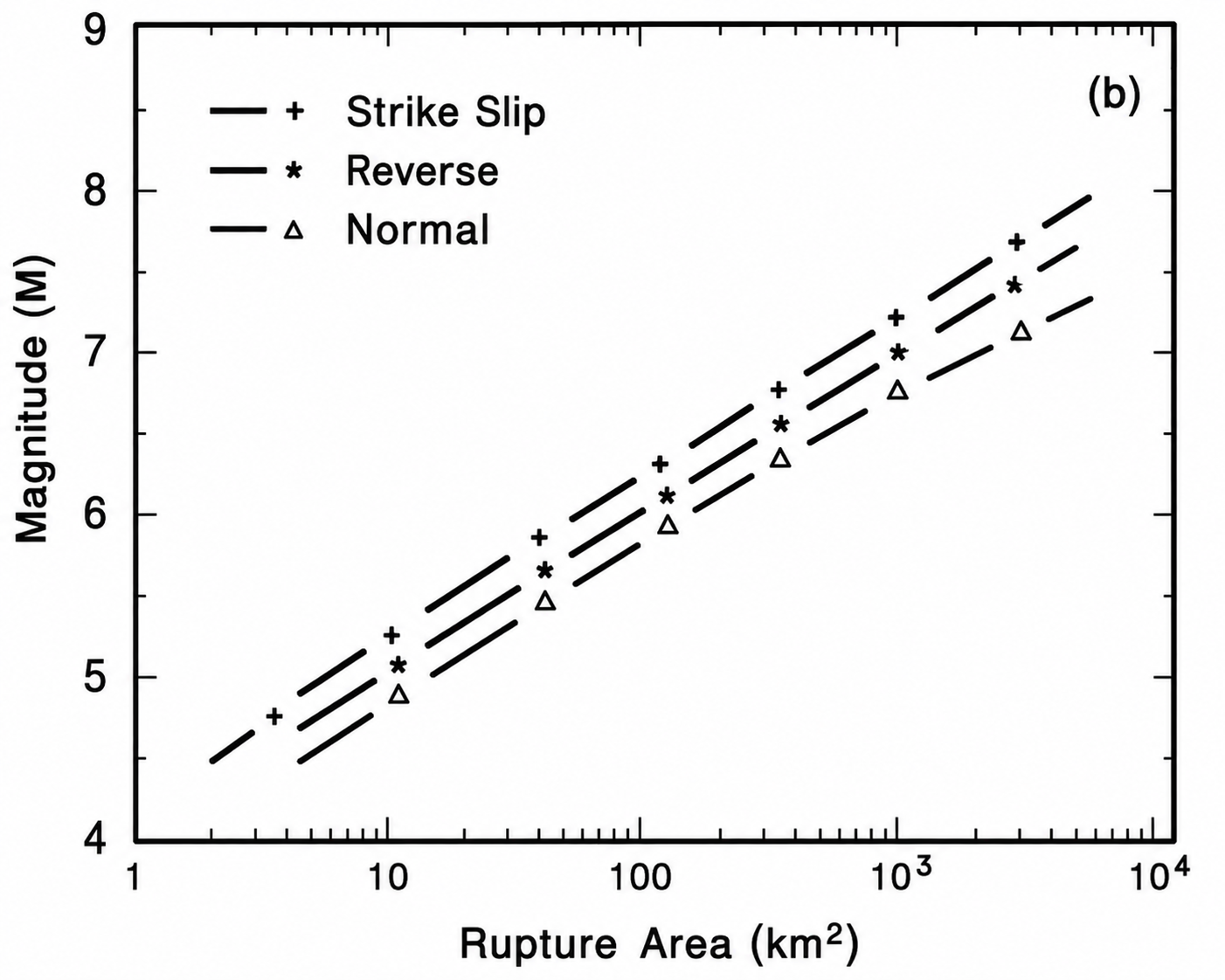 Fig. 16
Regression of rupture area on magnitude (M). Regression line shown for all-slip-type relationship. Short dashed line indicates 95% confidence interval. Regression lines for strike-slip, reverse, and normal-slip relationships. See Table 2 for regression coefficients. Length of regression lines shows the range of data for each relationship.
click on image to open in a new tab
Wells and Coppersmith (1994)
| Variable | Input | Units | Notes |
|---|---|---|---|
| km. | |||
| km. | |||
| Variable | Output | Units | Notes |
| unitless | Moment Magnitude computed using Wesnousky (2008) | ||
| unitless | Moment Magnitude computed using Hanks and Bakun (2008) | ||
| km.2 |
SEISMERIO - The Paleoseismic Scenarios Explorer
VS30 Site Effect
Slope Effect
Ridge Effect (aka Topographic Effect)
-
Figure 13a from
Massa et al (2010)
 Figure 13. (a)
Residuals between predicted acceleration response spectra (5% damping) for reference station (NRN2) and for station NRN7, for periods up to 1 s. The results are reported for the west—east component and are presented in terms of logarithmic differences. PGHA indicates peak ground horizontal component (in this case, the east—west component).
Massa et al (2010)
Site Effect is based on Equation 2 and Figure 13 a of
Figure 13. (a)Residuals between predicted acceleration response spectra (5% damping) for reference station (NRN2) and for station NRN7, for periods up to 1 s. The results are reported for the west—east component and are presented in terms of logarithmic differences. PGHA indicates peak ground horizontal component (in this case, the east—west component).
Massa et al (2010)
Radiation Patterns
- Fig. 2 Schematic map view
of the radiation pattern for a vertical strike-slip fault and its effect on near-fault ground displacements from Somerville et al. (1997)
 Fig. 2
Schematic map view of the radiation pattern for a vertical strike-slip fault and its effect on near-fault ground displacements.
Click on image to open in a new tab.
Somerville et al. (1997)> - Fig. 13 Empirical model
of the strike-normal to average horizontal response spectral ratio, showing its dependence on period and distance from Somerville et al. (1997)
 Fig. 13
Empirical model of the strike-normal to average horizontal response spectral ratio excluding dependence on the angles θ or φ, shown as a function of period for various magnitudes and distances (top), and as function of distance for various magnitudes and periods (bottom).
Click on image to open in a new tab.
Somerville et al. (1997)> - Fig. 17 Schematic diagram
of the polarity of permanent ground displacement for strike-slip earthquakes from Somerville et al. (1997)
 Fig. 17
Schematic diagram of the polarity of permanent ground displacement for strike-slip earthquakes. The motions are shown for both left-lateral and right-lateral unilateral faults, and for both northerly and southerly rupture propagation on north-striking faults.
Click on image to open in a new tab.
Somerville et al. (1997)>
Single-value calculator
| Variable | Input | Units | Notes |
|---|---|---|---|
| Magnitude (M) | Mw | Model valid for M > 6 | |
| Rupture Distance (r_rup) | km | Model tabulated for r_rup 0-50 km | |
| Period | sec | Restricted to periods tabulated in Table 6 | |
| Variable | Output | Units | Notes |
| FN/Average Ratio (Strike-Normal / Average) | ratio | Multiplier applied to average horizontal motion for strike-normal component | |
| Strike-Parallel / Average | ratio | Reciprocal of the strike-normal ratio |
Ratio vs period (fixed magnitude, several distances)
| Magnitude (M) |
FN/Average Ratio is the strike-normal component of horizontal ground motion divided by the average horizontal motion predicted by an attenuation relation (Somerville et al. 1997). r_rup is the closest distance from the site to the fault rupture, in km.
Ratio vs distance (fixed period, the four magnitudes used by Somerville et al. 1997)
| Period |
FN/Average Ratio is the strike-normal component of horizontal ground motion divided by the average horizontal motion predicted by an attenuation relation (Somerville et al. 1997). r_rup is the closest distance from the site to the fault rupture, in km.
- Fig. 9 Empirical model
of the response spectral amplitude ratio, showing its dependence on period and directivity function from Somerville et al. (1997)
 Fig. 9
Empirical model of the response spectral amplitude ratio, showing its dependence on period and on the directivity function (Xcos θ for strike-slip; Ycos φ for dip-slip).
Click on image to open in a new tab.
Somerville et al. (1997)>
Single-value calculator
| Variable | Input | Units | Notes |
|---|---|---|---|
| Magnitude (M) | Mw | Model valid for M > 6 | |
| Rupture Distance (r_rup) | km | Model tabulated for r_rup 0-50 km | |
| Period | sec | Restricted to periods tabulated in Table 6 | |
| Variable | Output | Units | Notes |
| FN/Average Ratio (Strike-Normal / Average) | ratio | Multiplier applied to average horizontal motion for strike-normal component | |
| Strike-Parallel / Average | ratio | Reciprocal of the strike-normal ratio |
Ratio vs period (fixed magnitude, several distances)
| Magnitude (M) |
FN/Average Ratio is the strike-normal component of horizontal ground motion divided by the average horizontal motion predicted by an attenuation relation (Somerville et al. 1997). r_rup is the closest distance from the site to the fault rupture, in km. This model does not distinguish between strike-slip and dip-slip mechanisms.
Ratio vs distance (fixed period, the four magnitudes used by Somerville et al. 1997)
| Period |
FN/Average Ratio is the strike-normal component of horizontal ground motion divided by the average horizontal motion predicted by an attenuation relation (Somerville et al. 1997). r_rup is the closest distance from the site to the fault rupture, in km. This model does not distinguish between strike-slip and dip-slip mechanisms.
Archaeoseismic Calculators
Rodkin and Korzhenkov (2018) presented two ways to estimate Peak Ground Velocity (PGV) - the Tilt Method (my name) and the PGV estimation method (PGVEM - their name).
Tilt Method
- Fig. 11 from Rodkin and Korzhenkov (2018) -
 Fig. 11
A sketch map showing the destruction of- an ideal rigid wall
- a more realistic wall composed of blocks of stones separated by joints
Rodkin and Korzhenkov (2018) - Figure 4 from
Korzhenkov and Mazor (2014) -
 Fig. 4
A tilt southward of the southern wall at the SE premises of the Northern Church (field station 3). The degree of the tilting is increasing with the distance from the abutted perpendicular wall. This phenomenon is the result of maximum freedom of oscillation at the central part of the wall
Korzhenkov and Mazor (2014)
| Structure | Height (m) | Thickness (m) | α - Critical Tilt Angle |
|---|---|---|---|
| Church | |||
| House |
PGV Estimation Method
- Fig. 13 from
Korzhenkov and Mazor (2014) -
 Fig. 13
A horizontal 15 cm shift eastward of the upper part of an arch column in one of the excavated quarters
Korzhenkov and Mazor (2014) - Figure 16 from
Korzhenkov and Mazor (2014) -
 Fig. 16
Clockwise rotation of a stone in an eastern wall (field station 9)
Korzhenkov and Mazor (2014)
Landslide Calculators
Static Analysis
A Factor of Safety (FS) for the slope is estimated first to determine if the slope was stable under aseismic conditions. Two methods are considered here - the Fellenius method and the modified Bishop method. Both methods divide the soil model into vertical slices and determine Factor of Safety as a ratio from a sum of moment balances performed on each vertical slice. This accounts for changes in topography and lateral changes in unit thicknesses and elevation of the water table. The generalized equation is shown below.FS = Σ Mr / Σ Md
where
Mr = Resisting Moment
Md = Driving Moment
Resisting Moment is the ability of the soil mass to avoid moving. The driving moment is the forces such as gravity and water saturated layers pushing the soil mass down slope. FS less than 1 indicates that the slope is unstable. FS greater than 1 indicates that the slope is stable. Factor of Safety tends to be sensitive to the height of the water table. Lower values of FS are associated with shallower water tables. If you know the time of year an earthquake struck, this could help you estimate the height of the water table. Well data can also be helpful. Ideally, mechanical tests on soil layers can inform your 2 model of the various layers. Wechsler et al (2009) used the commercial software Slope/W™ to perform the Static Analysis at Umm Qanatir.
Dynamic Analysis
The Newmark Displacement method can be used to evaluate slope stability during an earthquake. First a critical acceleration is estimated. Critical acceleration is the minimum earthquake induced acceleration that initiates slope movement. Critical acceleration is computed as follows:ac = (FS-1)sinβ
where
ac = critical acceleration measured in g's (1 g = 9.81 m/s2)
FS = Factor of Safety (computed previously for a range of conditions)
β = Thrust angle (degrees)
-
Newmark (1965)'s slope stability model
showing thrust angle (β)
 Fig. 15 a
O = Circle center
c.g. = Center of Gravity
β = Thrust angle
Newmark (1965)
lnDN = 1.521*ln(Iα) - 1.993ln(ac) - 1.546
where
DN = Newmark Displacement (cm.)
Iα = Arias Intensity (m/s)
ac = Critical acceleration (g's)
Arias Intensity (Iα) can be related to Magnitude and Fault Distance using an equation derived for the Dead Sea by Katz and Crouvi (2007):
log10Iα = 1.2MW - 2.2log10R - 4.9
where
Iα = Arias Intensity
MW = Moment Magnitude
R = Fault Distance (km.)
By assuming a DN of 5 or 10 cm., one can solve for Iα and then MW as a function of R.
-
Figure 13a from
Massa et al (2010)
Figure 13. (a) Residuals between predicted acceleration response spectra
(5% damping) for reference station (NRN2) and for station NRN7, for periods up to 1 s.
The results are reported for the west—east component and are presented in terms of logarithmic differences.
PGHA indicates peak ground horizontal component (in this case, the east—west component).
Massa et al (2010)
Site Effect is based on Equation 2 and Figure 13 a of
Figure 13. (a) Residuals between predicted acceleration response spectra
(5% damping) for reference station (NRN2) and for station NRN7, for periods up to 1 s.
The results are reported for the west—east component and are presented in terms of logarithmic differences.
PGHA indicates peak ground horizontal component (in this case, the east—west component).Massa et al (2010)
Tsunami Calculators
-
Bounding Envelopes for landslide tsunamis from
Salamon and Di Manna (2019)
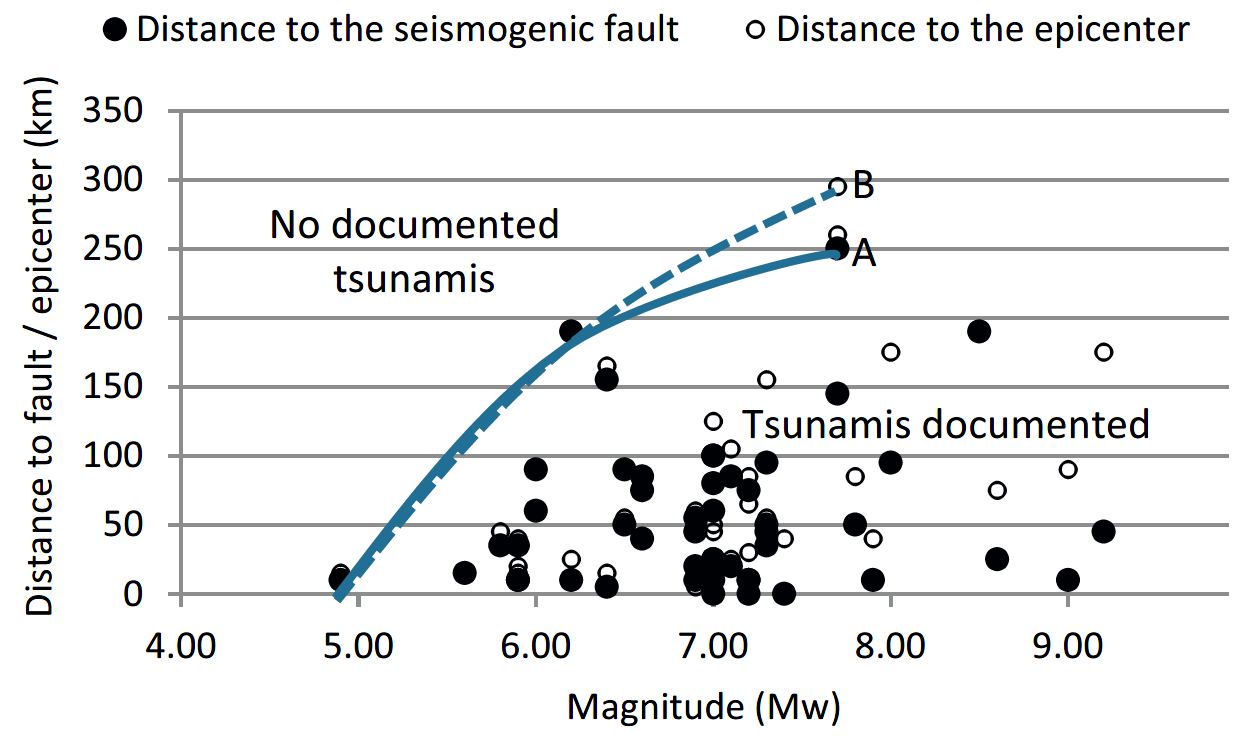 Fig. 4.
Empirical ‘Magnitude-Distance’ bounding envelopes for tsunamis generated by seismogenic submarine landslides. Filled circles denote the distance from the seismogenic fault to the landslide scar (Rf), and empty circles denote the distance between the earthquake epicenter and the landslide scar (Re). The bounding envelope of the maximal distance between the seismogenic fault and the landslide scar is delineated by line A and the bounding envelope between the epicenter and the landslide scar is denoted by the dashed line B.
Salamon and Di Manna (2019)
Seismite Calculators
Sand Boils
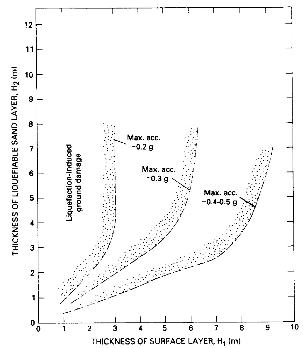
Fig. 9. - Proposed boundary curves relating thickness of nonliquefiable surface layer to thickness of the liquefiable zone as a function of peak earthquake accelerations required to induce venting or ground rupturing at the surface. From Ishihara (1985). Obermeier (1996)
| Variable | Input | Units | Notes |
|---|---|---|---|
| g | Peak Horizontal Ground Acceleration | ||
| Variable | Output (No Site Effect) |
Units | Notes |
| unitless | Conversion from PGA to Intensity using Wald et al (1999) |